A set of tools to help design a laboratory based prevalence study harnessing the pooling of laboratory samples to increase resource efficiency. The tools provide guidance in choosing the number of samples to pool and the total number of tests to perform, focusing on achieving the maximum estimation performance (low uncertainty and estimation error) while keeping the total amount of tests low. In the package there are functions to simulate study outcomes, optimize the study design, and finally, analyze the results of a pooled study to retrieve the prevalence estimates. The package is based on a Bayesian framework, with the possibility to perform a full hierarchical analysis including uncertainty due to the sensitivity in acquiring the testing material. The package was developed at the occasion of the COVID-19 pandemic, but can be utilized in every laboratory based prevalence study.
This package is produced as a companion to the following guidance from the European Center for Disease Prevention and Control: https://www.ecdc.europa.eu/sites/default/files/documents/Methodology-estimating-point-prevalence%20-SARS-CoV-2-infection-pooled-RT-PCR-testing.pdf.
You can install the released version of PooledPrevalence with:
# install.packages("devtools")
devtools::install_github("EU-ECDC/PooledPrevalence")The main goal of the package is to estimate prevalence in a
population/risk group, given the results of a pooled laboratory test.
Let’s assume a test with the following design: 2000 individual
biological samples divided in 10 samples per testing pool (pool size),
for a total of 200 pools. In this experiment we observe 30 positive
pools (15%). With get_estimates() it is possible to estimate the
underlying prevalence:
library(PooledPrevalence)

results <- get_estimates(10, 200, 30)

print(results$estimates)
#>   p_test  k        Est         Lo         Up
#> 1   0.15 30 0.01610737 0.01103635 0.02251263
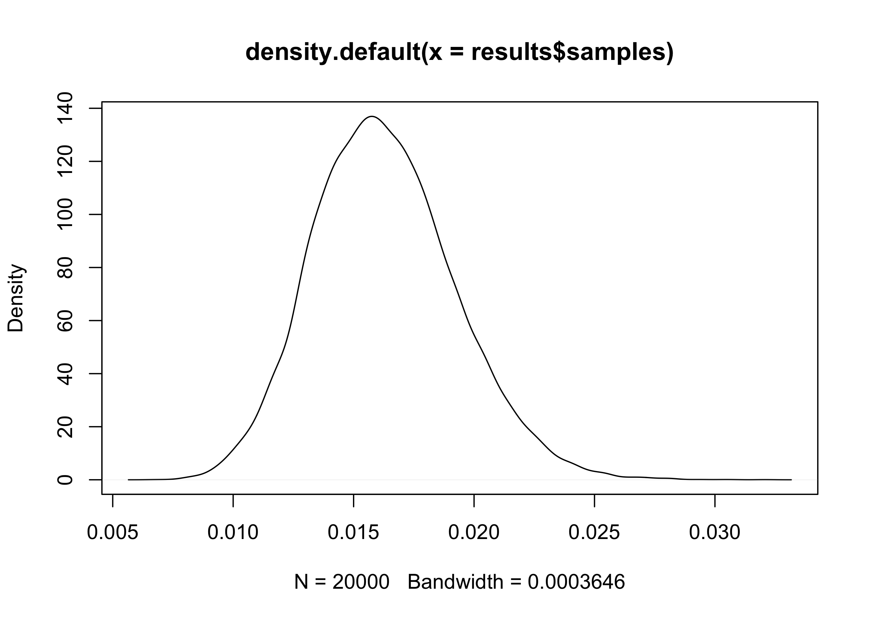
The object results contains both the estimates and, if a Bayesian
method is used, the posterior samples of the distribution. The samples
allows the inspection of the full posterior distribution of the
prevalence.
results <- get_estimates(10, 200, 30)

plot(density(results$samples))
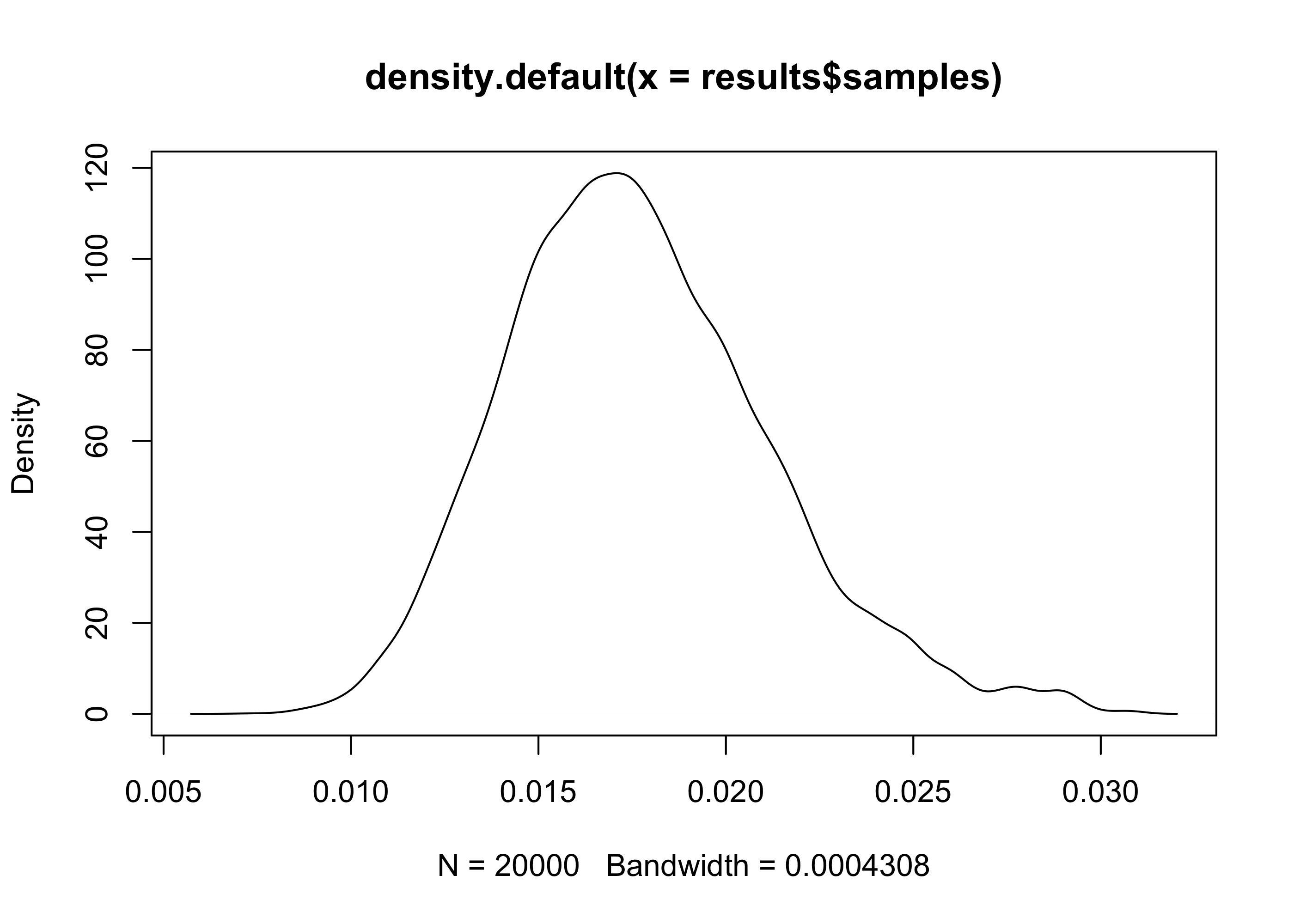
With Hierarchical Bayesian (HB) estimation is possible to account for the risk of false negatives due to incorrect sampling of material. Notice that the resulting estimates are therefore slightly higher. HB allows also a more correct evaluation of the uncertainty and should be the preferred method for the final analyses.
results <- get_estimates(10, 200, 30, method = 'HB')
#>
#>
#> @@@@@@@@@@@@@@@@@@@@@@@@@@@@@@@@@@@@@@@@@@@@@@@@@@@@@@@@@
#> The Metropolis acceptance rate was 0.75312
#> @@@@@@@@@@@@@@@@@@@@@@@@@@@@@@@@@@@@@@@@@@@@@@@@@@@@@@@@@

plot(density(results$samples))Having access to the posterior samples allows Bayesian hypothesis testing for decision making. For example, a public health authority may want to remove in a geographical region a certain control measure only if the average prevalence is below 2% with a > 90% probability:
results <- get_estimates(10, 200, 30, iters = 200000)

mean(results$samples < .02)
#> [1] 0.892735
In this case the probability of a mean prevalence below 2% is 89.3%, therefore there’s not enough evidence in favor of removing the control measure. We may want to increase the sample size of the study or wait more. The Bayesian framework allows to simply add new samples to the already collected ones and simply update the analysis.
old.results <- get_estimates(10, 200, 30, iters = 200000)

new.tested.pools <- 60

new.positve.pools <- 9

new.results <- get_estimates(10, 200 + new.tested.pools, 30 + new.positve.pools, iters = 200000)

mean(new.results$samples < .02)
#> [1] 0.92148
The new probability is 92.1%, so we have enough evidence to remove the control measure.
Finally, we want to ascertain the probability that region A, with 30 positive pools out of 200, has a lower prevalence or region B (38 positive pools out of 180).
region.A <- get_estimates(10, 200, 30, iters = 200000)

region.B <- get_estimates(10, 180, 38, iters = 200000)

mean(region.A$samples < region.B$samples)
#> [1] 0.94025The package provides a tool to help program the most efficient design for a prevalence study based on pooled testing. The methodology tries to maximize statistical accuracy while increasing the ratio between pool size and number of tests.
The user needs to specify the operational limits that are driven by the
available resources (number of sampled individuals n.max and maximum
number of laboratory test to perform w.max), the expected (maximal)
prevalence, and by the possible reduction in sensitivity due to an
excessive number of samples in the same pool (s.max). This number
depends on a number of factors (the pathogen, the sensitivity of the
test, the laboratory infrastructure and technique), therefore it needs
to be decided after appropriate local validation tests. A good starting
point for validation is between 10 and 20 samples per pool.
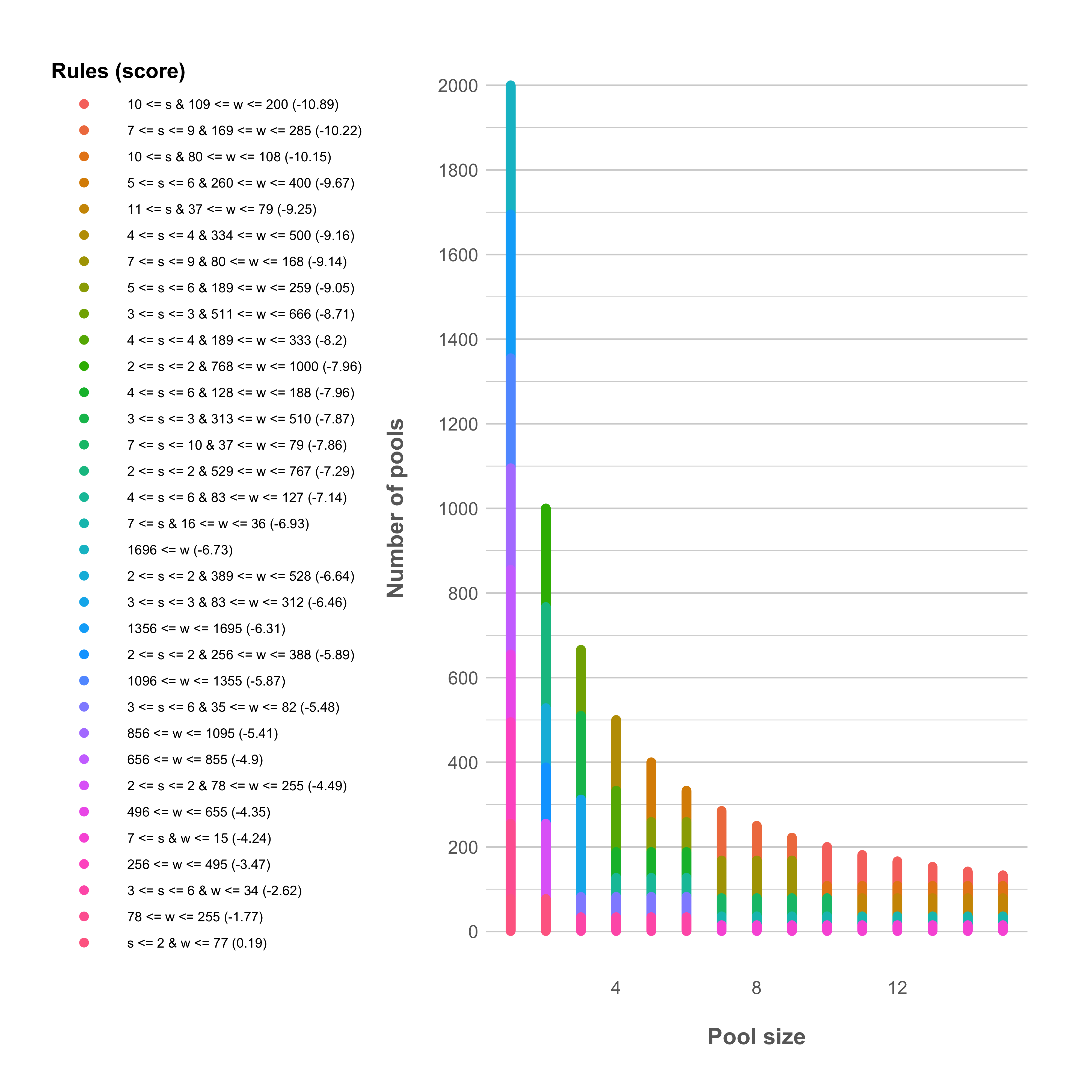
In the following example we investigate the possible designs for a study with a maximal pool size of 15 and a maximal number of tests and individuals to sample equal to 2000. We also set a maximal expected prevalence of 5%. Given the nature of pooled testing, the statistical accuracy decreases with the prevalence, so it is better to select a value which is higher than the prevalence we actually expect to find, in order not to end up with an underpowered study.
grid <- design_optimization(s.max = 15, w.max = 2000, p = .05, n.max = 2000)

plot_optimization_grid(grid)
The plot shows the “optimization windows” with different colors, ordered by the average score (lower is better).
We can observe that the best window (score: -10.89) is achieved with a
pool size s of 10 or more and with a number of test w higher than
108.
Once a window has been identified, simulation tests can be used to
evaluate the statistical performance. The tests need to be carried on
specific couples of values of pool size s and number of tests w.
In order to decrease the risk of sensitivity problems we suggest to
evaluate the more conservative designs in term of pool size (lower s),
but validation studies can allow to choose a higher value. Regarding the
number of tests, one should use the higher number that is achievable
during the study, since the higher the number of tests, the higher the
statistical precision; through pooling the maximum number of test needed
is already decreased by a factor equal to s (e.g. for s == 10, given
2000 individuals planned for sampling, at maximum 2000 / s = 200 tests
will be done).
Let’s compare the results in term of statistical accuracy using w = 109 and w = 200.
simulation.low_w <- simulate_pool_test(s = 10, w = 108, p = 0.05)

print(format_simulation(simulation.low_w))
#>                            [,1]
#> Estimated prevalence       "4.9%, 95%CI: [3.6%, 6.5%]"
#> Estimation uncertainty     "2.9%, 95%CI: [2.4%, 3.5%]"
#> Estimation error           "0.48%, 95%CI: [5e-04, 1.7%]"
#> Unpooled study prevalence  "5%, 95%CI: [3.7%, 6.3%]"
#> Unpooled study uncertainty "2.6%, 95%CI: [2.3%, 2.9%]"
#> Unpooled study error       "0.46%, 95%CI: [2.7e-05, 1.5%]"

simulation.high_w <- simulate_pool_test(s = 10, w = 200, p = 0.05)

print(format_simulation(simulation.high_w))
#>                            [,1]
#> Estimated prevalence       "5%, 95%CI: [4%, 6.2%]"
#> Estimation uncertainty     "2.2%, 95%CI: [1.9%, 2.5%]"
#> Estimation error           "0.38%, 95%CI: [0.021%, 1.2%]"
#> Unpooled study prevalence  "5%, 95%CI: [4.1%, 6%]"
#> Unpooled study uncertainty "1.9%, 95%CI: [1.7%, 2.1%]"
#> Unpooled study error       "0.35%, 95%CI: [1.5e-05, 1.1%]"
It is possible to see that in both simulations the statistical accuracy
of the pooled design is similar to that achieved through an unpooled
study (e.g. s_unpooled = 1 and w_unpooled = w * s). Instead, it’s
possible to observe a definite decrease in uncertainty and error passing
from 108 to 200 tests. In any case, both numbers are definitely lower
than than the 2000 tests that would have been performed wihout pooling.


