This package contains a suite of functions for recovering dive records from 1970’s film-based Kooyman-Billups Time Depth Records (KBTDRs). This TDR was among the first placed on a free-ranging marine organism, but the film-based format of the behavioral data makes long-term comparisons exceptionally challenging. This package returns a corrected, continuous, and digitized file of a KBTDR record complete with dates, times, and depth that can be easily read into dive analysis software.
There are eight main recovery steps that are achieved in this package:
- Record digitization (completed manually in ImageJ)
- Scan centering
- Arc removal
- Zero offset correction
- X-axis transformation to dates & times
- Interpolation between missing points
- Y-axis transformation to depth
- Spline smoothing
You can install the package from GitHub:
# load the development version:
devtools::install_github("EmmaLiTsai/recoverKBTDR")
library(recoverKBTDR)This is a basic example of the intended workflow for historic record recovery:
Step one: read in data (trace and time dots) after scan image processing, which contains the X and Y values of the record in centimeters from the origin:
# examples of data tidying from raw ImageJ csv files:
filepath <- system.file("extdata", "WS_25_1981", package = "recoverKBTDR")
filepath_trace <- paste(filepath, "WS_25_1981_trace.csv", sep = "/")

tidy_trace <- tidy_raw_trace(filepath_trace)
head(tidy_trace)
## x_val y_val
## 1 0.190 0.624
## 2 0.190 0.611
## 3 0.312 0.652
## 4 0.312 0.624
## 5 0.312 0.611
## 6 0.312 0.570
# showing tidy data that is included within the package:
data(trace)
head(trace)
## # A tibble: 6 × 2
## x_val y_val
## <dbl> <dbl>
## 1 0.19 0.624
## 2 0.19 0.611
## 3 0.312 0.652
## 4 0.312 0.624
## 5 0.312 0.611
## 6 0.312 0.57
data(time_dots)
head(time_dots)
## # A tibble: 6 × 2
## x_val y_val
## <dbl> <dbl>
## 1 1.73 -0.279
## 2 3.23 -0.294
## 3 4.65 -0.302
## 4 6.07 -0.314
## 5 7.50 -0.331
## 6 8.91 -0.354
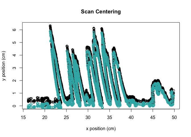
Step two: center the record using the timing dots, such that all timing dots will be centered along y = -center_along_y. After centering, it is recommended that you also extract the centered psi calibration curve (if available) such that the data correctly align with the centered dive record. This helps remove drift in alignment due to record scanning:
# centering along y = -0.9:
trace <- center_scan(trace, time_dots, center_along_y = 0.9)

# visualizing the centered record:
plot(tidy_trace[1000:11000,], xlab = "x position (cm)", ylab = "y position (cm)", type = "p", main = "Scan Centering")
points(trace[1000:11000,], col = "#39b3b2")
# also extract the centered psi calibration curve:
psi_calibration <- centered_psi_calibration(trace, psi_interval = c(100, 200, 400, 600, 800))
head(psi_calibration)## psi_interval psi_position
## 1 100 1.689131
## 2 200 3.749440
## 3 400 8.321658
## 4 600 13.440813
## 5 800 18.414504
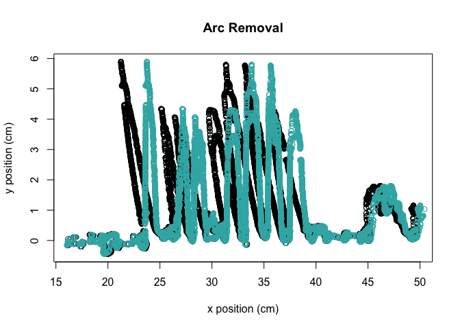
Step three: Remove the left-leaning arc across the record created by the KBTDR arm. This function removes the curvilinear nature of the original record, such that it becomes a function.
# Here, center_y is the height of transducer arm pivot point. This value is usually close to 11 cm, but there is slight variation between devices
trace <- remove_arc(trace, center_y = 11.1)
# to find the center_y value for arc removal, check out the helper function ?find_center_y()

# visualizing this correction:
plot(trace[1000:11000, 1:2], xlab = "x position (cm)", ylab = "y position (cm)", type = "p", main = "Arc Removal")
points(trace[1000:11000, c(3,2)], col = "#39b3b2")
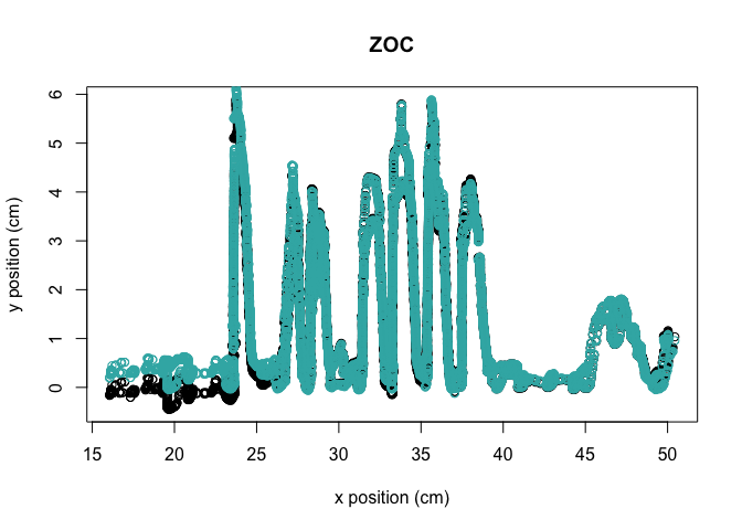
Step four: some records present extreme drift and/or level shifts in surface values. This drift is common with modern TDRs and can be resolved using zero-offset correction methods modeled after the “diveMove” package. Code had to be modified from this package to handle the uncorrected trace data frame. These methods can be used with the zoc() function:
trace_zoc <- zoc(trace, k_h  = 500, depth_bounds = c(-1, 1))

# visualizing this correction:
plot(trace[1000:11000,c(3,2)],xlab = "x position (cm)", ylab = "y position (cm)", type = "p", main = "ZOC")
points(trace_zoc[1000:11000,c(3,4)], col = "#39b3b2")
Step five: transform the x-axis into minutes using the timing dots (often placed 12 minutes apart)
# removing the data frame and also transform the x-axis to time in minutes from the origin.
trace <- transform_x_vals(trace,
                          time_dots,
                          time_period_min = 12)
head(trace)
## x_val y_val new_x time
## 1 0.190 -0.010 0.1838265 1.275097
## 2 0.190 0.003 0.1918505 1.330755
## 3 0.339 -0.132 0.2568894 1.781892
## 4 0.326 -0.105 0.2607944 1.808979
## 5 0.353 -0.146 0.2621015 1.818045
## 6 0.353 -0.132 0.2708894 1.879001
Step six: the seal often moved faster than the LED arm could document the dive during the descent and ascent phases. The function add_dates_times() uses the trace data frame to create POSIXct date time objects, and also interpolates between missing values to create a more regular time series. This helps with future spline smoothing and dive analysis.
trace <- add_dates_times(trace,
                         start_time = "1981:01:16 15:10:00",
                         on_seal = "1981:01:16 17:58:00",
                         off_seal = "1981:01:23 15:30:00",
                         tz = "Antarctica/McMurdo")
# now, the record is complete with POSIXct date times:
head(trace)
## date_time x_val y_val new_x time interp_y
## 1 1981-01-16 17:58:00 19.710 0.010 19.71617 168.0015 0.01000000
## 2 1981-01-16 17:58:01 19.696 0.037 19.71878 168.0257 0.03700000
## 3 1981-01-16 17:58:02 19.723 -0.004 19.72053 168.0419 -0.00400000
## 4 1981-01-16 17:58:03 NA NA NA NA 0.00950000
## 5 1981-01-16 17:58:04 19.710 0.023 19.72417 168.0756 0.02300000
## 6 1981-01-16 17:58:05 NA NA NA NA 0.01866667
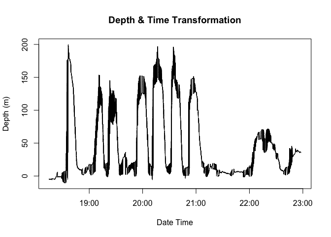
Step seven: transform y-axis to depth either using the maximum depth or psi calibration curve (if available):
# If psi calibration curve is present:
trace <- transform_y_vals(trace, psi_calibration = psi_calibration, max_psi = 900, max_position = 22.45)

# If we just know max depth:
trace_maxdep <- transform_y_vals(trace, max_dep = 319)

# visualizing this transformation:
plot(trace[1000:18000, c(1,8)],xlab = "Date Time", ylab = "Depth (m)", type = "l", main = "Depth & Time Transformation")
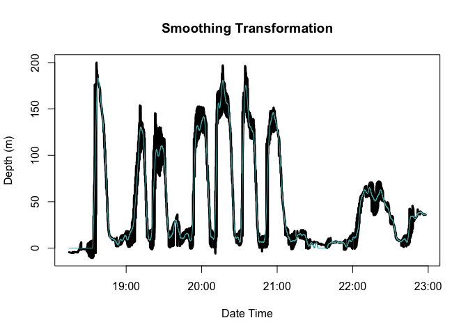
Step eight: spline smoothing is done to reduce noise in the data by passing the spar value and depth threshold (in meters) to use when a dive is detected:
# smoothing the data frame with a rolling mean depth threshold of 5, and a spar value of 0.3 when a dive is detected:
trace <- smooth_trace_dive(trace, spar_h = 0.3, depth_thresh = 5)

# seeing how smoothing preformed:
{plot(trace[1000:18000, c(1,8)], xlab = "Date Time", ylab = "Depth (m)", type = "l", main = "Smoothing Transformation", lwd = 3)
lines(trace[1000:18000, c(1,9)], col = "#39b3b2")
}
# to find the best spar value for spline smoothing, check out the helper function ?find_best_spar() Then, final data frame can be exported and read into dive analysis software.
library(recoverKBTDR)
## basic example code
data(trace)
data(time_dots)

# centering the data
trace <- center_scan(trace, time_dots, center_along_y = 0.9)

# extracting the centered psi calibration curve, if needed:
psi_calibration <- centered_psi_calibration(trace, psi_interval = c(100, 200, 400, 600, 800))

# remove the arc:
trace <- remove_arc(trace, center_y = 11.1)

# time assignment
trace <- transform_x_vals(trace, time_dots, time_period_min = 12)

# POSIXct date times and interpolating
trace <- add_dates_times(trace, start_time = "1981:01:16 15:10:00", on_seal = "1981:01:16 17:58:00", off_seal = "1981:01:23 15:30:00", tz = "Antarctica/McMurdo")

# add depths
trace <- transform_y_vals(trace, psi_calibration = psi_calibration, max_psi = 900, max_position = 22.45)

# spline smoothing
trace <- smooth_trace_dive(trace, spar_h = 0.3, depth_thresh = 5)

# export!

# fast recovery can also be used, where an argument csv file is used to quickly pass arguments to the functions above. For use, check out the ?fast_recovery(filepath)

