Nixtla

Statistical ⚡️ Forecast

Lightning fast forecasting with statistical and econometric models

StatsForecast offers a collection of widely used univariate time series forecasting models, including exponential smoothing and automatic ARIMA modeling optimized for high performance using numba.

🔥 Highlights

Fastest and most accurate auto_arima in Python and R.
New!: Replace FB-Prophet in two lines of code and gain speed and accuracy. Check the experiments here.
New!: Distributed computation in clusters with ray. (Forecast 1M series in 30min)
New!: Good Ol' sklearn syntax with AutoARIMA().fit(y).predict(h=7).

🎊 Features

Inclusion of exogenous variables and prediction intervals.
Out of the box implementation of exponential smoothing, croston, seasonal naive, random walk with drift and tbs.
20x faster than pmdarima.
1.5x faster than R.
500x faster than Prophet.
Compiled to high performance machine code through numba.
1,000,000 series in 30 min with ray.

Missing something? Please open an issue or write us in

📖 Why?

Current Python alternatives for statistical models are slow and inaccurate. So we created a library that can be used to forecast in production environments or as benchmarks. StatsForecast includes an extensive battery of models that can efficiently fit thousands of time series.

🔬 Accuracy

We compared accuracy and speed against: pmdarima, Rob Hyndman's forecast package and Facebook's Prophet. We used the Daily, Hourly and Weekly data from the M4 competition.

The following table summarizes the results. As can be seen, our auto_arima is the best model in accuracy (measured by the MASE loss) and time, even compared with the original implementation in R.

dataset	metric	nixtla	pmdarima [1]	auto_arima_r	prophet
M4-Daily	MASE	3.26	3.35	4.46	14.26
M4-Daily	time	1.41	27.61	1.81	514.33
M4-Hourly	MASE	0.92	---	1.02	1.78
M4-Hourly	time	12.92	---	23.95	17.27
M4-Weekly	MASE	2.34	2.47	2.58	7.29
M4-Weekly	time	0.42	2.92	0.22	19.82

[1] The model auto_arima from pmdarima had problems with Hourly data. An issue was opened in their repo.

The following table summarizes the data details.

group	n_series	mean_length	std_length	min_length	max_length
Daily	4,227	2,371	1,756	107	9,933
Hourly	414	901	127	748	1,008
Weekly	359	1,035	707	93	2,610

⏲ Computational efficiency

We measured the computational time against the number of time series. The following graph shows the results. As we can see, the fastest model is our auto_arima.

Nixtla vs Prophet

You can reproduce the results here.

External regressors

Results with external regressors are qualitatively similar to the reported before. You can find the complete experiments here.

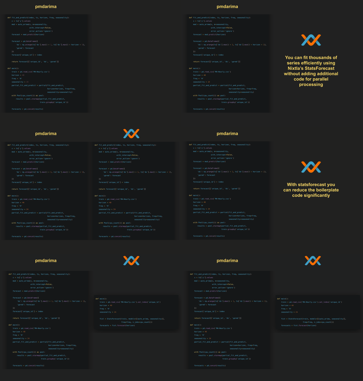
👾 Less code

📖 Documentation

Here is a link to the documentation.

🧬 Getting Started

Example Jupyter Notebook

💻 Installation

PyPI

You can install the released version of StatsForecast from the Python package index with:

pip install statsforecast

(Installing inside a python virtualenvironment or a conda environment is recommended.)

Conda

Also you can install the released version of StatsForecast from conda with:

conda install -c conda-forge statsforecast

(Installing inside a python virtualenvironment or a conda environment is recommended.)

Dev Mode

If you want to make some modifications to the code and see the effects in real time (without reinstalling), follow the steps below:

git clone https://github.com/Nixtla/statsforecast.git
cd statsforecast
pip install -e .

🧬 How to use

The following example needs ipython and matplotlib as additional packages. If not installed, install it via your preferred method, e.g. pip install ipython matplotlib.

import numpy as np
import pandas as pd
from IPython.display import display, Markdown

import matplotlib.pyplot as plt
from statsforecast import StatsForecast
from statsforecast.models import seasonal_naive, auto_arima
from statsforecast.utils import AirPassengers

horizon = 12
ap_train = AirPassengers[:-horizon]
ap_test = AirPassengers[-horizon:]

series_train = pd.DataFrame(
    {
        'ds': pd.date_range(start='1949-01-01', periods=ap_train.size, freq='M'),
        'y': ap_train
    },
    index=pd.Index([0] * ap_train.size, name='unique_id')
)

fcst = StatsForecast(
    series_train, 
    models=[(auto_arima, 12), (seasonal_naive, 12)], 
    freq='M', 
    n_jobs=1
)
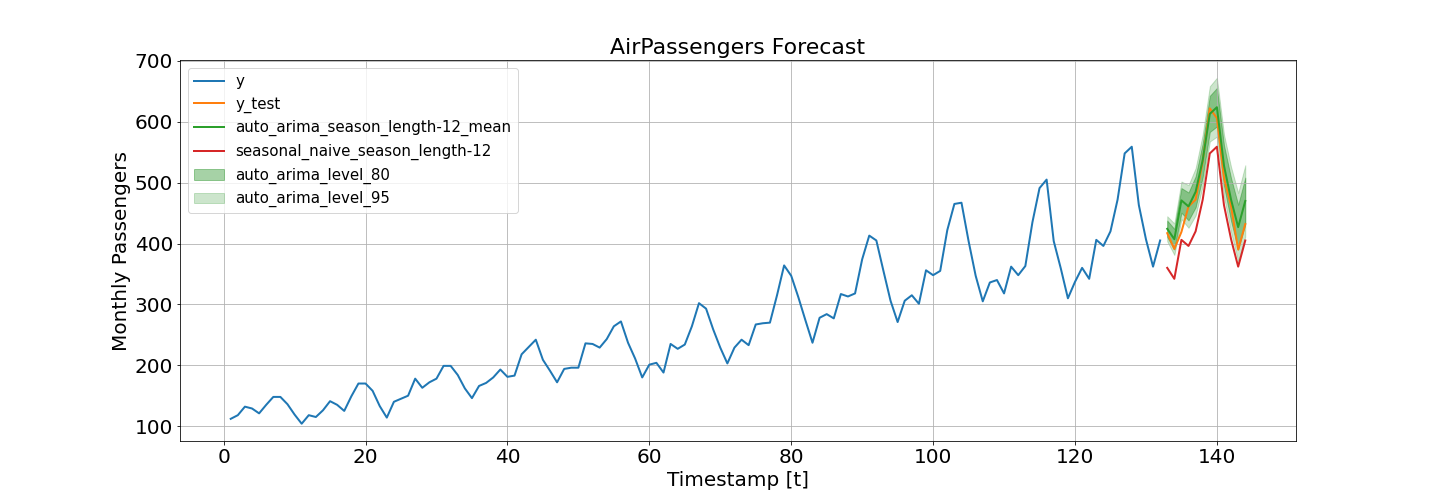
forecasts = fcst.forecast(12, level=(80, 95))

forecasts['y_test'] = ap_test

fig, ax = plt.subplots(1, 1, figsize = (20, 7))
df_plot = pd.concat([series_train, forecasts]).set_index('ds')
df_plot[['y', 'y_test', 'auto_arima_season_length-12_mean', 'seasonal_naive_season_length-12']].plot(ax=ax, linewidth=2)
ax.fill_between(df_plot.index, 
                df_plot['auto_arima_season_length-12_lo-80'], 
                df_plot['auto_arima_season_length-12_hi-80'],
                alpha=.35,
                color='green',
                label='auto_arima_level_80')
ax.fill_between(df_plot.index, 
                df_plot['auto_arima_season_length-12_lo-95'], 
                df_plot['auto_arima_season_length-12_hi-95'],
                alpha=.2,
                color='green',
                label='auto_arima_level_95')
ax.set_title('AirPassengers Forecast', fontsize=22)
ax.set_ylabel('Monthly Passengers', fontsize=20)
ax.set_xlabel('Timestamp [t]', fontsize=20)
ax.legend(prop={'size': 15})
ax.grid()
for label in (ax.get_xticklabels() + ax.get_yticklabels()):
    label.set_fontsize(20)

Adding external regressors

series_train['trend'] = np.arange(1, ap_train.size + 1)
series_train['intercept'] = np.ones(ap_train.size)
series_train['month'] = series_train['ds'].dt.month
series_train = pd.get_dummies(series_train, columns=['month'], drop_first=True)

display_df(series_train.head())

ds	y	trend	intercept	month_2	month_3	month_4	month_5
1949-01-31 00:00:00	112	1	1	0	0	0	0
1949-02-28 00:00:00	118	2	1	1	0	0	0
1949-03-31 00:00:00	132	3	1	0	1	0	0
1949-04-30 00:00:00	129	4	1	0	0	1	0
1949-05-31 00:00:00	121	5	1	0	0	0	1

xreg_test = pd.DataFrame(
    {
        'ds': pd.date_range(start='1960-01-01', periods=ap_test.size, freq='M')
    },
    index=pd.Index([0] * ap_test.size, name='unique_id')
)

xreg_test['trend'] = np.arange(133, ap_test.size + 133)
xreg_test['intercept'] = np.ones(ap_test.size)
xreg_test['month'] = xreg_test['ds'].dt.month
xreg_test = pd.get_dummies(xreg_test, columns=['month'], drop_first=True)

fcst = StatsForecast(
    series_train, 
    models=[(auto_arima, 12), (seasonal_naive, 12)], 
    freq='M', 
    n_jobs=1
)
forecasts = fcst.forecast(12, xreg=xreg_test, level=(80, 95))

forecasts['y_test'] = ap_test

🔨 How to contribute

See CONTRIBUTING.md.

📃 References

The auto_arima model is based (translated) from the R implementation included in the forecast package developed by Rob Hyndman.

Contributors ✨

Thanks goes to these wonderful people (emoji key):

_fede 💻	_{José Morales} 💻 🚧	_{Sugato Ray} 💻	_{Jeff Tackes} 🐛	_darinkist 🤔	_{Alec Helyar} 💬	_{Dave Hirschfeld} 💬
_mergenthaler 💻	_Kin 💻	_Yasslight90 🤔	_asinig 🤔	_{Philip Gillißen} 💻	_{Sebastian Hagn} 🐛