To install this package use the following steps. You’ll need the package
remotes installed first, skip to the second step if you already have
it.
install.packages("remotes") #install remotes
remotes::install_github("ashenoy-cmbi/grafify@*release", dependencies = T) #install latest release with dependencies
grafify depends on ggplot2, lmerTest, emmeans, car,
pbkrtest, tidyr, purrr and Hmisc packages.
The main goals of this package, besides making it easier for me to share data and functions for the statistics workshop, are the following:
- easily make common types of graphs based on
ggplot2but with fewer lines of code - carry out ANOVA analysis using linear models (
lm) and mixed effects (lmer) - perform post-hoc comparisons (through
emmeans) - simulate one-way and two-way ANOVA design data for power analysis
If you’re interested in basic theory and code for stats in R, also visit Statistics for Micro/Immuno Biologists.
grafify has four main kinds of functions as follows.
-
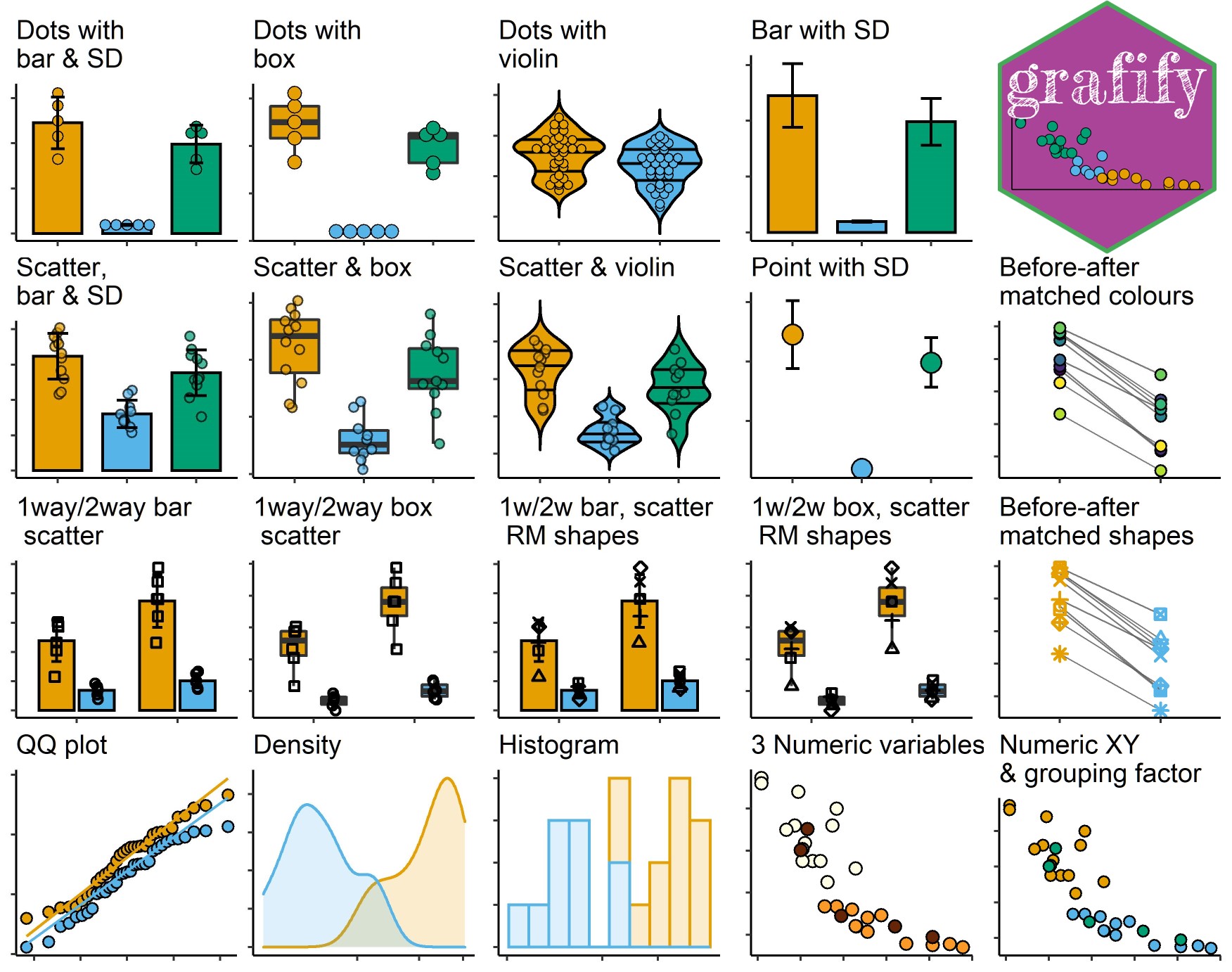
There are 19
plot_functions of 6 broad types ingrafify. Theplot_scatter..versions are preferred when there are many data points,plot_dot..versions have a “cleaner” layout for smaller datasets.- Two categorical variables: these graphs either use scatter (or
also called jitter) or dot plot geometries:
plot_scatterbar_sd,plot_scatterbox,plot_scatterviolinandplot_dotbar_sd,plot_dotbox,plot_dotviolin - Three or four categorical variables:
plot_3d_scatterbar,plot_3d_scatterbox,plot_4d_scatterbar,plot_4d_scatterbox - Quantitative X-Y & a third variable:
plot_xy_NumGroup,plot_xy_CatGroup - Matched before-after graphs:
plot_befafter_colours,plot_befafter_shapes - Data distributions:
plot_qqline,plot_densityplot_histogram - Summary graphs with SD error bars:
plot_bar_sd,plot_point_sd
- Two categorical variables: these graphs either use scatter (or
also called jitter) or dot plot geometries:
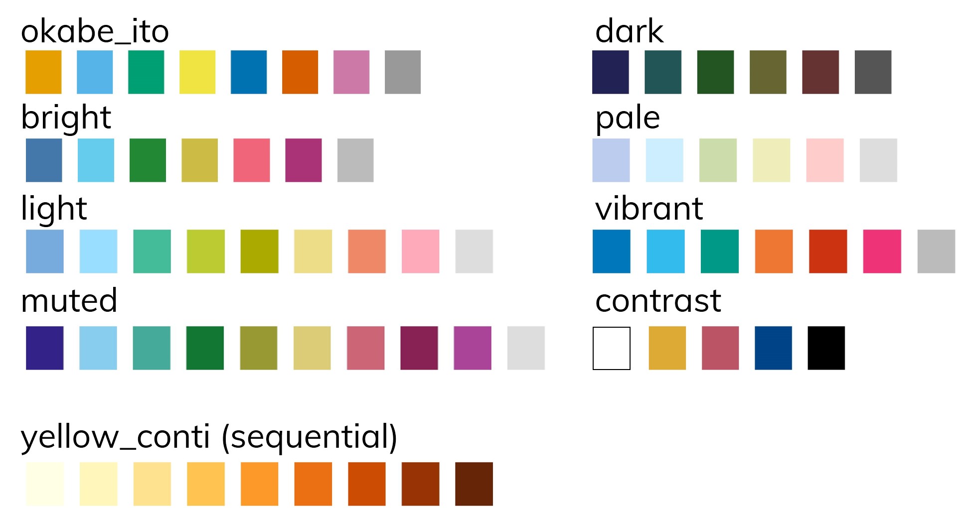
The following qualitative and continuous palettes are implemented in
grafify:
(The continuous colour scheme based on Paul Tol’s YlOrBl variant is new in v0.2.0.)
-
Fitting linear models and linear mixed models and obtaining ANOVA tables
- linear models for ordinary ANOVAs:
simple_anova,simple_model, - linear mixed effects ANOVAs:
mixed_anova,mixed_model
- linear models for ordinary ANOVAs:
-
Perform post-hoc comparisons based on fitted models
posthoc_Pariwiseposthoc_Levelwiseposthoc_vsRef
-
Generating random one-way and two-way data based on mean and SD.
- one-way designs:
make_1way_data,make_1way_rb_data - two-way designs:
make_2way_data,make_2way_rb_data
- one-way designs:
-
Colour-blind compatible schemes:
Visit the grafify vignettes
website for detailed examples of usage.
Full reference to all functions available at grafify
pages.
This version “breaks” a few arguments from v0.3.1, therefore is v1.4.1.
Specifically, opacity for both symbols and bars/boxes/violins can be set
using s_alpha and b_alpha or v_alpha, respectively; previously,
only bars/boxes/violin opacity could be set with a single alpha
parameter. Old code with just alpha will no longer work, sorry! There
are also new graph types and arguments for ANOVAs as below.
-
New graph types
plot_densityandplot_histogramfor smooth density or histogram plots throughgeom_densityandgeom_histogramrespectively.- two new plot types
plot_scatterboxandplot_scatterviolinthat complement theplot_dot...versions and instead usegeom_pointwithposition_jitter. These versions are useful when a large number of data points are needed to be plotted.
-
Updates
simple_anovawhere the table also has Mean SS.mixed_anovanow has two new arguments, one to change method for Df calculation and second to get type I or III SS (default is type II).jitterargument added toplot_3d..andplot_4d..functions for consistency with other scatter plots.bwidargument (for adjusting width of bars) added toplot_scatterbar_sdfor consistency.
Bug fixes in mixed_model and simple_model which now correctly lists
the data used in the call field.
- A new
plot_4d_scatterbarfunction which is likeplot_4d_scatterboxbut plots bar and SD. So there are now twoplot_3d_andplot_4d_functions. - Text on X-axis on all graphs can be rotated from 0-90 using
TextXAngleargument to prevent overlap. plot_dot_functions now havedotthickoption to set stroke thickness. This is similar tosymthickfor scatter/jitter plots.- Using
facet_wraporfacet_gridwill not draw a box around panel text (unlike the default intheme_classic()). plot_3d_andplot_4d_functions draw symbols in black colour.
- Bug fixes in
plot_3d_scatterbarandplot_3d_scatterbox, which now correctly use the “shapes” variable to fill colour of bars/boxes and shape of the symbols; symbols are depicted in black. simple_anovagenerates type II ANOVA table throughcar::Anova(), so thecarpackage is now a dependency. v0.1.0 and v0.2.0 generated type I ANOVA table throughstats::anova().
- the main difference from v0.1.0 is that all
plot_functions apply theall_grafifycolour scheme by default (seeplot_vignettes on how to change colours) - two new types of graphs are possible with two quantitative X-Y plots
with a third variable that is either numeric (
plot_xy_NumGroup) or categorical (plot_xy_CatGroup). - there are two new continuous colour schemes (
scale_fill_grafify_candscale_colour_grafify_c), based on Paul Tol’s variant of YlOrBl scheme.


