

Tablesaw is the shortest path to data science in Java. It includes a dataframe, an embedded column-store, and hundreds of methods to transform, summarize, or filter data similar to the Pandas dataframe and R data frame. If you work with data in Java, it will probably save you time and effort.
Tablesaw also supports descriptive statistics, data visualization, and machine learning. And it scales: You can munge a 1/2 billion rows on a laptop and over 2 billion records on a server.
There are other, more elaborate platforms for data science in Java. They're designed to work with vast amounts of data, and require a huge stack and a vast amount of effort.
You can include tablesaw-core, which is the dataframe library itself, with:
<dependency>
    <groupId>tech.tablesaw</groupId>
    <artifactId>tablesaw-core</artifactId>
    <version>0.11.0</version>
</dependency>
You may also add dependencies for tablesaw-plot to use the plotting capability and tablesaw-smile to use the Smile machine learning integration.
- Please see our documentation page: https://jtablesaw.github.io/tablesaw/
- We also recommend trying Tablesaw inside Jupyter notebooks, which lets you experiment with Tablesaw in a more interactive manner. Get started by installing BeakerX and trying the sample Tablesaw notebook
- Import data from RDBMS and CSV files, local or remote (http, S3, etc.)
- Combine files
- Add and remove columns
- Sort, Group, Filter
- Map/Reduce operations
- Store tables in a fast, compressed columnar storage format
- Descriptive stats: mean, min, max, median, sum, product, standard deviation, variance, percentiles, geometric mean, skewness, kurtosis, etc.
- Regression: Least Squares
- Classification: Logistic Regression, Linear Discriminant Analysis, Decision Trees, k-Nearest Neighbors, Random Forests
- Clustering: k-Means, x-Means, g-Means
- Association: Frequent Item Sets, Association Rule Mining
- Feature engineering: Principal Components Analysis
- Scatter plots
- Line plots
- Vertical and Horizontal Bar charts
- Histograms
- Box plots
- Quantile Plots
- Pareto Charts
Here's an example where we use XChart to map the locations of tornadoes:
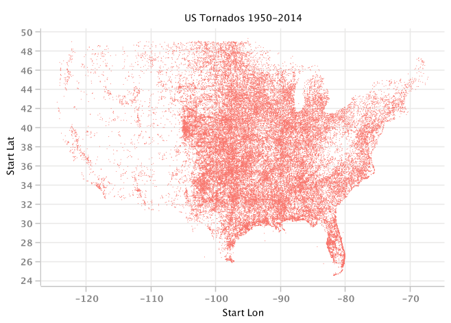
You can see examples and read more about plotting in Tablesaw here: https://jtablesaw.wordpress.com/2016/07/30/new-plot-types-in-tablesaw/.
You can load a 500,000,000 row, 4 column csv file (35GB on disk) entirely into about 10 GB of memory. If it's in Tablesaw's .saw format, you can load it in 22 seconds. You can query that table in 1-2 ms: fast enough to use as a cache for a Web app.
BTW, those numbers were achieved on a laptop.
The goal in this example is to identify the production shifts with the worst performance. These few lines demonstrate data import, column-wise operations (differenceInSeconds()), filters (isInQ2()) grouping and aggegating (median() and .by()), and (top(n)) calculations.
Table ops = Table.read().csv("data/operations.csv");                             // load data
DateTimeColumn start = ops.dateColumn("Date").atTime(ops.timeColumn("Start"));
DateTimeColumn end = ops.dateColumn("Date").atTime(ops.timeColumn("End");
LongColumn duration = start.differenceInSeconds(end);                            // calc duration
duration.setName("Duration");
ops.addColumn(duration);

Table filtered = ops.selectWhere(                                                // filter
    allOf(
        column("date").isInQ2(),
        column("SKU").startsWith("429"),
        column("Operation").isEqualTo("Assembly")));

Table summary = filtered.median("Duration").by("Facility", "Shift");             // group medians
FloatArrayList tops = summary.floatColumn("Median").top(5);                      // get "slowest"
If you see something that can be improved, please let us know.