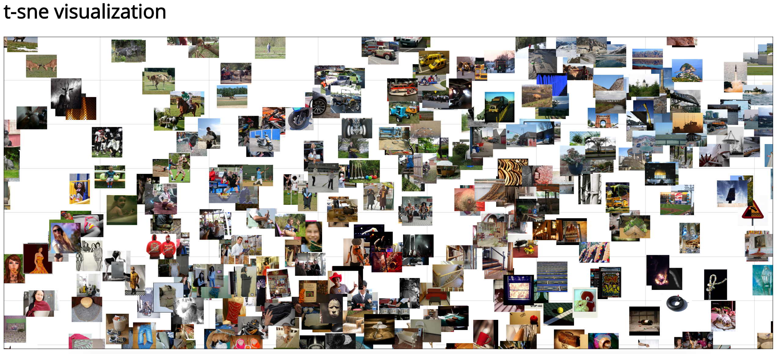
Visualize high dimensional data with t-sne using D3 and Python
pip install numpy
pip install tsne
pip install cherrypy
pip install jinja2- Put your images into the
public/data/folder. - Create a text file
images_list.txtsomewhere that contains your images in each line. For instance, runls public/data/ | shuf > images_list.txt. - Create a numpy file
data.npythat contains an NxM array where N = number of images and each row corresponds to the image inimages_list.txt, and M = number of features. For instance, extract CNN features for each image, put it into a numpy array and save to file:
import numpy as np
# N = number of images, M = feature dimension
data = np.array((N, M))
# ... put features into data ...
np.save('data.npy', data)First, preprocess your data with t-sne. This preprocessing step converts your high dimensional data into 2D via t-sne dimensionality reduction:
python preprocess_with_tsne.py /path/to/data.npy /path/to/images_list.txtwhere
data.npyis a numpy file with number of rows equal to the number of images and number of columns equals the number of featuresimages_list.txtis a text file with each row containing the file name of the image corresponding to the row of the numpy array
After this preprocessing script is run, it should output public/data.csv. This is required for the visualization to work.
Next, visualize your preprocessed data via
python visualize_2d_data.py --port 8080 --host 0.0.0.0Open your browser and go to localhost:8080. You should see your data visualized! Pan around by dragging with your mouse and zoom with your mouse's scroll wheel.
The server can look at multiple datasets. The default data file is public/data.csv and images folder is public/data. However, one can point to an arbitrary data file name public/XYZ.csv' and its corresponding images folder public/XYZ', and then pass the file name as a query string to the server: localhost:8080/?data=XYZ.
