The goal of ggsomewhere (and it’s github repository) is to provide tools for building spatial ggplot2 extensions.
The approach makes use of ggplot2’s sf plotting capabilities, the sf2stat package to prepare reference data for use inside a stat_* or geom_* layer, and the knitrExtra package functions for managing functions from a readme and working with template functions included in the readme.
How you’d use sf2stat to build functionality with scope, region type, and location name. When using the code templates for this north carolina county example, we’ll be replacing ‘scope’, ‘region’, and ‘locations’ as follows
- ‘scope’ -> ‘northcarolina’
- ‘region’ -> ‘county’
- ‘locations’ -> a vector of region names
Let’s see how we might recreate the functionality in the ggnorthcarolina package using some templates in this readme.
In the example, the scope of the package is ‘northcarolina’. The region of interest is ‘county’, and the location names that we are using are the county names.
devtools::create(".")usethis::use_data_raw()The reference data should have just the id columns and the geometry. Then it should be named similar to this:
geo_reference_northcarolina_county
Where ‘northcarolina’ is is the character string that will replace ‘scope’ when using the code templates, and ‘county’ is the character string that will replace region in the
nc <- sf::st_read(system.file("shape/nc.shp", package="sf"))
#> Reading layer `nc' from data source
#>   `/Library/Frameworks/R.framework/Versions/4.4-x86_64/Resources/library/sf/shape/nc.shp'
#>   using driver `ESRI Shapefile'
#> Simple feature collection with 100 features and 14 fields
#> Geometry type: MULTIPOLYGON
#> Dimension:     XY
#> Bounding box:  xmin: -84.32385 ymin: 33.88199 xmax: -75.45698 ymax: 36.58965
#> Geodetic CRS:  NAD27

geo_reference_northcarolina_county <- nc |>
  dplyr::select(county_name = NAME, fips = FIPS) |>
  sf2stat:::sf_df_prep_for_stat(id_col_name = "county_name")
#> Warning in st_point_on_surface.sfc(sf::st_zm(dplyr::pull(sf_df, geometry))):
#> st_point_on_surface may not give correct results for longitude/latitude data
#> Warning: The `x` argument of `as_tibble.matrix()` must have unique column names if
#> `.name_repair` is omitted as of tibble 2.0.0.
#> ℹ Using compatibility `.name_repair`.
#> ℹ The deprecated feature was likely used in the sf2stat package.
#>   Please report the issue to the authors.
#> This warning is displayed once every 8 hours.
#> Call `lifecycle::last_lifecycle_warnings()` to see where this warning was
#> generated.

usethis::use_data(geo_reference_northcarolina_county, overwrite = T)
#> ✔ Setting active project to '/Users/evangelinereynolds/Google Drive/r_packages/ggsomewhere'
#> ✔ Saving 'geo_reference_northcarolina_county' to 'data/geo_reference_northcarolina_county.rda'
#> • Document your data (see 'https://r-pkgs.org/data.html')knitrExtra:::chunk_to_dir("nc_geo_reference_prep",
dir = "data-raw/")knitrExtra:::chunk_variants_to_dir(chunk_name = "stat_region_template",
file_name = "stat_county.R",
replace1 = "scope",
replacements1 = "northcarolina",
replace2 = "region",
replacements2 = "county")
#> It seems you are currently knitting a Rmd/Qmd file. The parsing of the file will be done in a new R session.compute_panel_scope_region <- function(data,
scales,
keep_id = NULL,
drop_id = NULL,
stamp = FALSE){
if(!stamp){data <- dplyr::inner_join(data, geo_reference_scope_region)}
if( stamp){data <- geo_reference_scope_region }
if(!is.null(keep_id)){ data <- dplyr::filter(data, id_col %in% keep_id) }
if(!is.null(drop_id)){ data <- dplyr::filter(data, !(id_col %in% drop_id)) }
data
}
# step 2
StatSfscoperegion <- ggplot2::ggproto(`_class` = "StatSfscoperegion",
`_inherit` = ggplot2::Stat,
# required_aes = c("fips|county_name"),
compute_panel = compute_panel_scope_region,
default_aes = ggplot2::aes(label = after_stat(id_col)))
stat_region <- function(
mapping = NULL,
data = NULL,
geom = ggplot2::GeomSf,
position = "identity",
na.rm = FALSE,
show.legend = NA,
inherit.aes = TRUE,
crs = "NAD27", # "NAD27", 5070, "WGS84", "NAD83", 4326 , 3857
...) {
c(ggplot2::layer_sf(
stat = StatSfscoperegion, # proto object from step 2
geom = geom, # inherit other behavior
data = data,
mapping = mapping,
position = position,
show.legend = show.legend,
inherit.aes = inherit.aes,
params = rlang::list2(na.rm = na.rm, ...)
),
coord_sf(crs = crs,
default_crs = sf::st_crs(crs),
datum = crs,
default = TRUE)
)
}source("./R/stat_county.R")
library(ggplot2)
nc <- sf::st_read(system.file("shape/nc.shp", package="sf"))
#> Reading layer `nc' from data source
#> `/Library/Frameworks/R.framework/Versions/4.4-x86_64/Resources/library/sf/shape/nc.shp'
#> using driver `ESRI Shapefile'
#> Simple feature collection with 100 features and 14 fields
#> Geometry type: MULTIPOLYGON
#> Dimension: XY
#> Bounding box: xmin: -84.32385 ymin: 33.88199 xmax: -75.45698 ymax: 36.58965
#> Geodetic CRS: NAD27
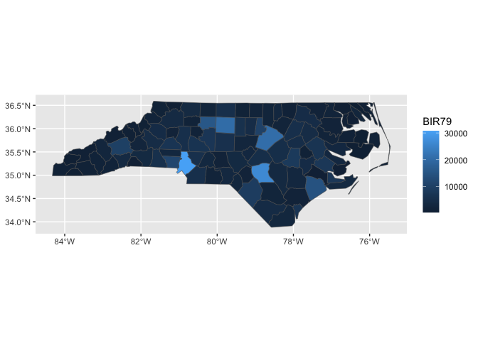
nc |>
sf::st_drop_geometry() |>
ggplot() +
aes(fips = FIPS) +
stat_county() +
aes(fill = BIR79)
#> Joining with `by = join_by(fips)`knitrExtra:::chunk_variants_to_dir(chunk_name = "geom_region_template",
file_name = "geom_county.R",
replace1 = "region",
replacements1 = "county")
#> It seems you are currently knitting a Rmd/Qmd file. The parsing of the file will be done in a new R session.geom_region <- stat_region
geom_region_label <- function(...){stat_region(geom = "text",...)}
stamp_region <- function(...){
stat_region(stamp = T,
data = mtcars,
aes(fill = NULL, color = NULL, label = NULL,
fips = NULL, region_name = NULL),
...)}
stamp_region_label <- function(...){
stat_region(stamp = T,
geom = "text",
data = mtcars,
aes(fill = NULL, color = NULL,
fips = NULL, region_name = NULL),
...)}source("./R/geom_county.R")
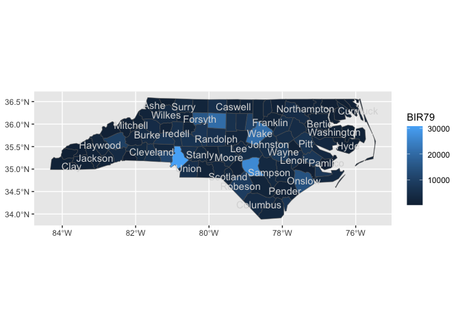
nc |>
sf::st_drop_geometry() |>
ggplot() +
aes(fips = FIPS) +
geom_county() +
geom_county_label(check_overlap = T,
color = "grey85") +
aes(fill = BIR79)
#> Joining with `by = join_by(fips)`
#> Joining with `by = join_by(fips)`last_plot() +
stamp_county() +
stamp_county_label()
#> Joining with `by = join_by(fips)`
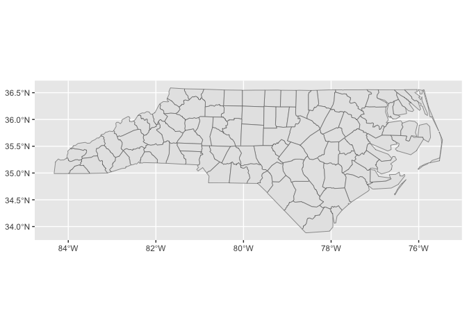
#> Joining with `by = join_by(fips)`ggplot() +
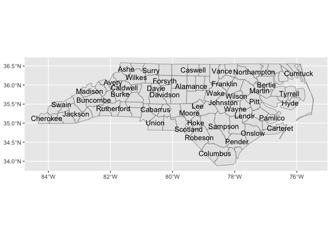
stamp_county()last_plot() +
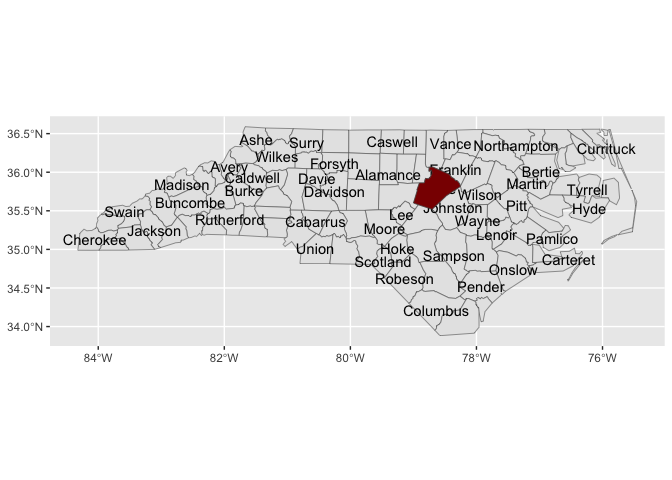
stamp_county_label(check_overlap = T)last_plot() +
stamp_county(keep_id = "Wake", fill = "darkred")locations <- geo_reference_northcarolina_county$county_name
locations_snake <- tolower(locations) |>
stringr::str_replace_all(" ", "_")
knitrExtra:::chunk_variants_to_dir(chunk_name = "stamp_region_location",
file_name = "stamp_county_location.R",
replace1 = "region",
replacements1 = rep("county", length(locations)),
replace2 = "location",
replacements2 = locations_snake,
replace3 = "Location",
replacements3 = locations)#' Title
#'
#' @param ...
#'
#' @return
#' @export
#'
#' @examples
stamp_region_location <- function(...){stamp_region(keep_id = 'Location', ...)}
#' Title
#'
#' @param ...
#'
#' @return
#' @export
#'
#' @examples
stamp_region_label_location <- function(...){stamp_region_label(keep_id = 'Location', ...)}source("./R/stamp_county_location.R")
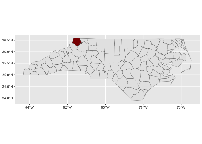
nc |>
sf::st_drop_geometry() |>
ggplot() +
aes(fips = FIPS) +
stamp_county() +
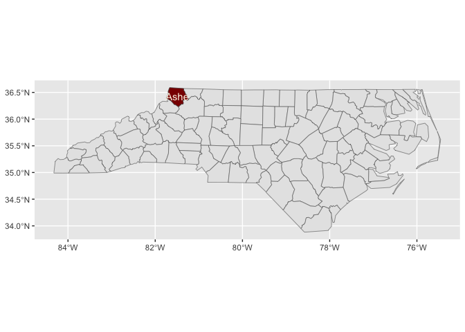
stamp_county_ashe(fill = "darkred")last_plot() +
stamp_county_label_ashe(color = "oldlace")