The Wearables Development Toolkit (WDK) is a set of tools to facilitate the development of activity recognition applications with wearable devices. It supports the following activities:
git clone https://github.com/avenix/WDK.git- install Matlab 2019a or greater.
- in Matlab, open the repository and type:
addpath(genpath('./'))in the console - use the Apps in each directory (e.g. AnnotationApp in 1-Annotation/).
- install the Signal Processing Toolbox by clicking on the Get More Apps button on Matlab's toolbar.
- to avoid issues with pathing, Matlab's current path should be set to the root of the WDK directory:
- the './data' directory should contain the following files and directories defined in the Constants.m file:
kLabelsPath = './data/annotations/labels.txt';
kAnnotationsPath = './data/annotations';
kMarkersPath = './data/markers';
kDataPath = './data/rawdata';
kCachePath = './data/cache';
kLabelGroupingsPath = './data/labeling';
kARChainsPath = './data/ARChains';
kVideosPath = './data/videos';
The Data Conversion App can be used to do a first check on the data after its collection. It offers the following features:
- Load any tabularized .txt data file and save it to the binary format used by the rest of the toolkit.
- Check whether there has been data loss using a user-specified timestamp signal and sampling interval.
- Visualize the different signals.
Note: by default, the Data Conversion App loads data files from the ./data/rawdata/ directory. Converted files are saved to the ./ root directory.
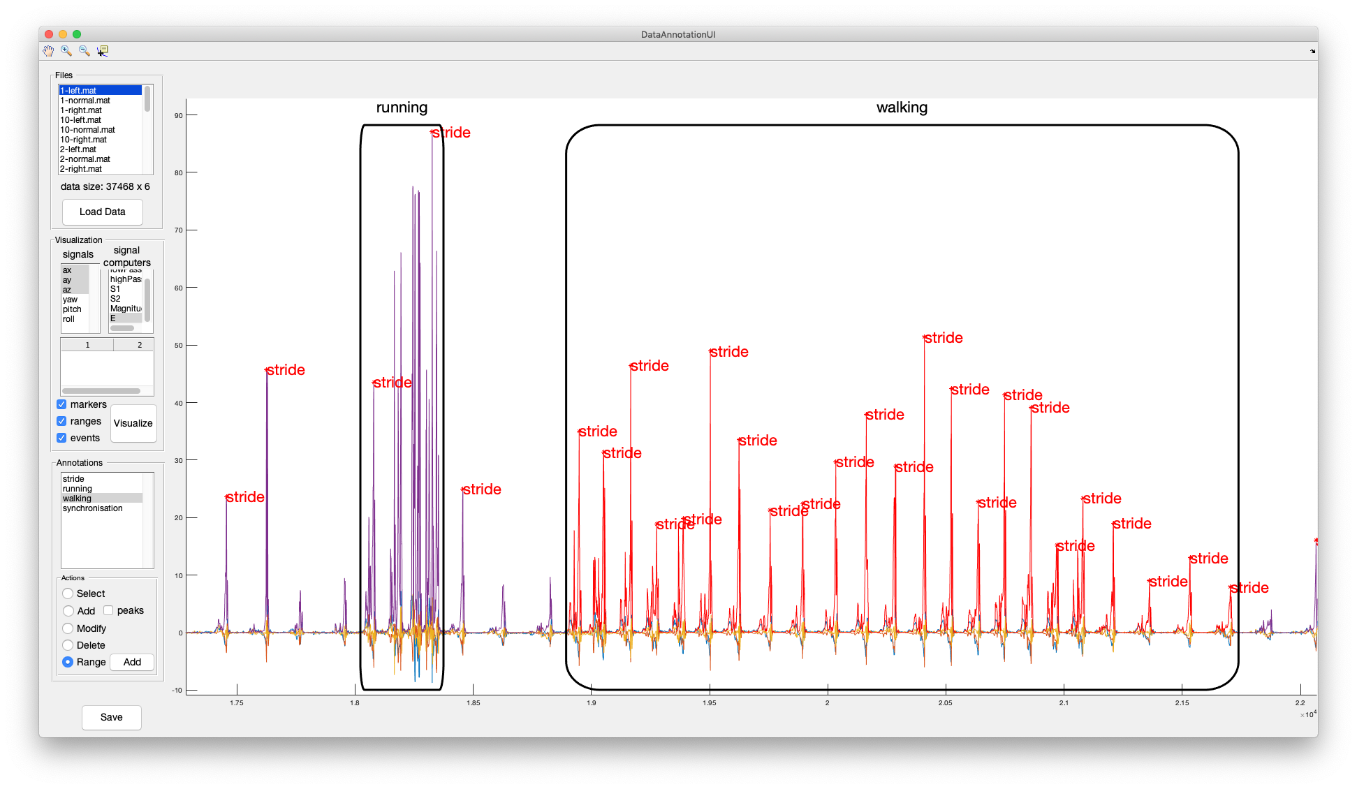
An annotated data set is needed to train a machine learning algorithm and to assess its performance. The Data Annotation App offers functionality to annotate time series data. Depending on the particular application, one might want to annotate events that occurr at a specific moment in time or activities that have a duration in time, called ranges. The following image shows the squared magnitude of the accelerometer signal collected by a motion sensor attached at a hind leg of a cow. The individual strides of the cow have been annotated as event annotations (red) and the walking and running activities as ranges (black rectangles).
The Data Annotation App can load and display videos next to the data. The video is synchronised to the data by matching two data samples to two video frames as defined in a synchronisation file. The format of a synchronisation file is:
sample1: 49727
sample2: 450209
frame1: 3302
frame2: 45284
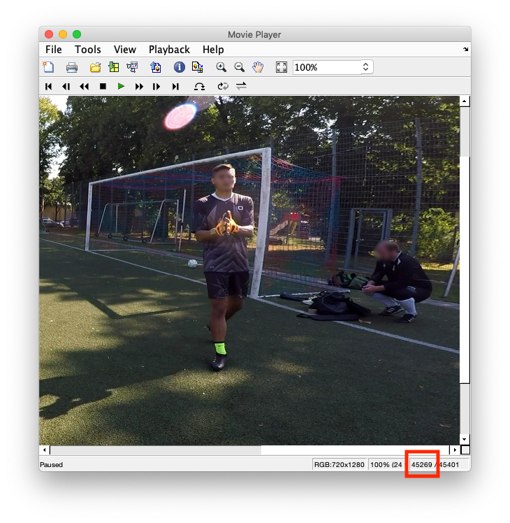
The exact frames of a specific event in a video are displayed on the Movie Player at the bottom right of the window:
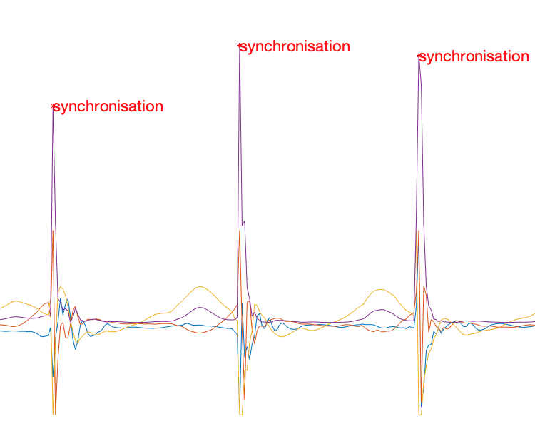
In this application, we asked the subject to applaud three times in front of the camera while wearing an armband with an Inertial Measurement Unit (IMU). We visualized the peak energy (i.e. squared magnitude) of the accelerometer signal and annotated each applause with the synchronisation label. When a data samples is selected on the plot, its timestamp is printed on Matlab's console. We copy the first synchronisation timestamp to the sample1 field of the synchronisation file. We do the same for the sample with timestamp 450209. The respective annotated synchronisation events are shown in the following image:
Please note:
- The Data Annotation App synchronises video and data at two points and interpolates linearly inbetween. We recommend the synchronisation points to take place in the beginning and end of a recording.
- Annotation, marker, synchronisation and video files should be consistent with the data files. If a data file is named 'S1.mat', its annotation file should be named 'S1-annotations.txt', its marker file 'S1-markers.edl', its synchronisation file 'S1-synchronisation.txt' and the video 'S1-video.videoFormat'.
- By default, the Data Annotation App loads annotation files from the './data/annotations/', video and synchronisation files from './data/videos' directory. Saved annotation files are located in the root './' directory.
- The labels to annotate should be defined in the 'labels.txt' file beforehand.
- You can use the keyboard shortcuts arrow-right, arrow-left and spacebar to iterate through data and video.
The Data Annotation App can import and display reference markers on top of the time series data. Currently, the Data Annotation App supports marker files created with the video annotation tool DaVinciResolve in .edl format. Markers added to a timeline in DaVinciResolve can be exported by: right-clicking on the Timeline -> timelines -> export -> Timeline markers to .EDL...:
In order to synchronise video markers and time series data, the .edl file should contain a synchronisation marker in the beginning and another one in the end of the file. Currently, the first and last green marker are matched to the first and last event annotation with the label synchronisaton. In order to annotate data:
- Annotate the video using DaVinci Resolve. Use a green marker to annotate a special event, ideally in the beginning and end of the file. (e.g. the user shakes the sensor three times in front of the camera).
- Export the markers to an .edl file.
- Copy the .edl file to the data/markers/ directory.
- Open the Data Annotation App and add an event annotation of the class synchronisation to the timestamp that corresponds .
- Reopen the Data Annotation App. This time the markers should be properly aligned with the data.
- Annotate the time series data.
Note: markers in .edl format are read from the './data/markers' directory.
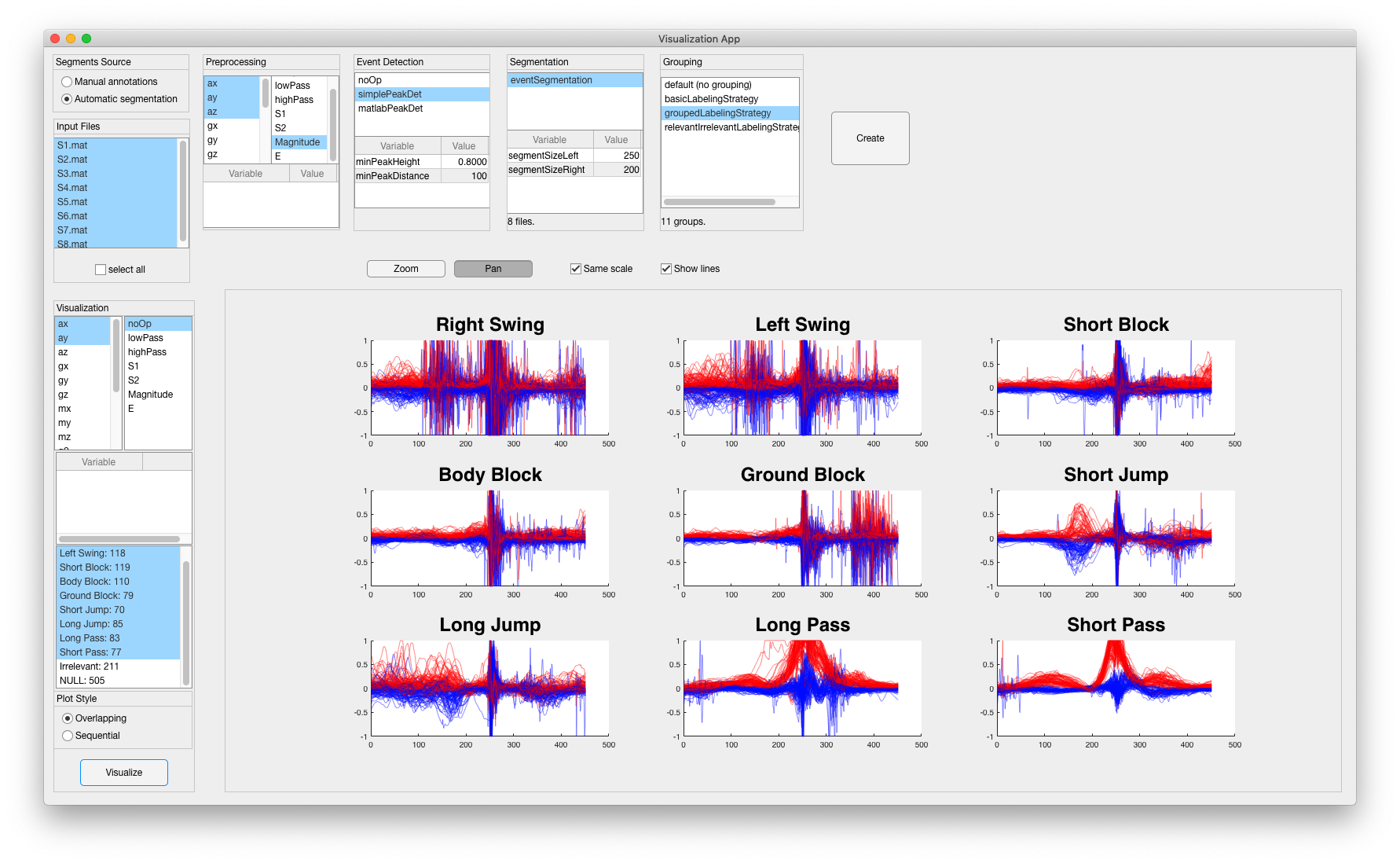
The Data Visualization App displays segments of data grouped by class. This is useful to study the differences across classes (e.g. to design an event detection or feature extraction algorithm). Segments can be plotted either on top of each other or sequentially (i.e. after each other). In order to visualize data:
- Select one or more input data files.
- Select where the segments should come from. Manual annotations creates segments from the range annotations and loads event annotations to create segments using the ManualSegmentationStrategy. The Automatic segmentation uses a preprocessing, event detection and segmentation algorithms selected over the user interface to create segments.
- (in Automatic segmentation mode) Select the signals to use, a preprocessing algorithm and (optionally) an event detection algorithm.
- Select a segmentation strategy and (optionally) a grouping strategy. Click the Create button. At this point the segments are created. A grouping strategy maps annotated labels to classes, usually by grouping different labels into classes.
- Select signals and classes to visualize and a plot style (i.e. overlapping or sequential).
Most wearable device applications execute a chain (i.e. sequence) of computations in order to detect specific patterns based on sensor signals. This chain of computations is called the Activity Recognition Chain and consists of the following stages:

Applications in the WDK can be developed visually over WDK-RED, via the user interface provided by the different WDK Apps, or directly via code.
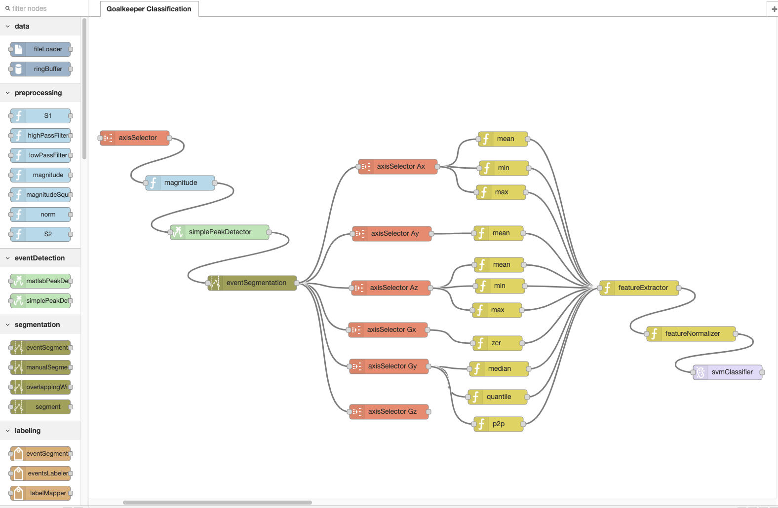
Activity recognition applications can be developed visually in Node-RED using the nodes available in the WDK-RED platform. The following image shows an activity recognition chain for detecting and classifying soccer goalkeeper training exercises using a wearable motion sensor attached to a glove worn by a goalkeeper:
Activity Recognition Chains can be imported and executed in the WDK as follows:
- Export the Activity Recognition Chains as described here.
- Execute the convertJSONToWDK.m script.
- Use the Execute from File button in each App.
Activity recognition applications can be developed directly in Matlab as long as the WDK is in Matlab's path. The Computer class is the superclass of every reusable component. Every Computer has the following properties and methods:
inputPort; %type of the input this computer takes
outputPort; %type of the output this computer produces
nextComputers; %array of computers this computer is connected to
output = compute(obj,input); %the method executed when this computer is visited (implemented in each subclass)
The following text snippet creates a chain of computations and saves it to the goalkeeperChain.mat file. This chain of computations detects events using a peak detector on the squared magnitude (sometimes called energy) of the accelerometer signal, segments the data around the detected events (200 samples to the left of the event and 30 sampels to the right) and extracts the features defined in the goalkeeperFeatureChain.mat file.
axisSelector = AxisSelector(1:3);%AX AY AZ
magnitudeSquared = MagnitudeSquared();

simplePeakDetector = SimplePeakDetector();
simplePeakDetector.minPeakHeight = single(0.8);
simplePeakDetector.minPeakDistance  = int32(100);

eventSegmentation = EventSegmentation();
eventSegmentation.segmentSizeLeft = 200;
eventSegmentation.segmentSizeRight = 30;

labeler = EventSegmentsLabeler();

featureExtractor = DataLoader.LoadComputer('goalkeeperFeatureChain.mat');

arcChain = Computer.ComputerWithSequence({FileLoader(),PropertyGetter('data'),...
axisSelector,magnitudeSquared,simplePeakDetector,eventSegmentation,labeler,...
featureExtractor});

DataLoader.SaveComputer(arcChain,'goalkeeperChain.mat');
This chain of computations produces a feature table that can be used within the Assessment App to study the performance of different machine learning algorithms.
Here you can find a list of the reusable components, their configurable properties and their performance metrics relative to an input of size n.
Invocations to preprocessing algorithms produce n values. The memory consumption of most preprocessing algorithms is 1 if the inPlaceComputation property is set to true or n otherwise.
| Name | Description | Flops | Memory |
|---|---|---|---|
| SimplePeakDetector | Threshold-based peak detector. Properties are: minPeakheight and minPeakDistance. Note: this algorithm is more suitable for deployment into an embedded device than the MatlabPeakDetector | 11 n | 1 |
| MatlabPeakDetector | Matlab's peak detector. Properties are: minPeakheight and minPeakDistance. | 1787 n | n |
Note: The flops metrics shown above have been calculated with random values in the range [0 1] using minPeakHeight = 0.8, minPeakDist = 100. The performance metrics will vary depending on how often peaks are detected based on the input data and minPeakHeight and minPeakDist properties.
The event detection algorithms output a single value.
An invocation to an event detection algorithm produces 0 or 1 value.
| Name | Description | Flops | Memory |
|---|---|---|---|
| SlidingWindow | Creates a segment of size segmentSize after every sampleInterval samples. E.g. segmentSize = 200 and sampleInterval = 100 creates segments with a 50% overlapping. Note: receives a signal as input. | segmentSize | segmentSize |
| EventSegmentation | Creates a segment around an event by taking segmentSizeLeft samples to the left and segmentSizeRight to the right of the event. Note: receives an event as input. | segmentSizeLeft + segmentSizeRight | segmentSizeLeft + segmentSizeRight |
| ManualSegmentation | Creates segments for each annotation (converts RangeAnnotations to segments and creates segments around each EventAnnotations). This segmentation strategy cannot be used in a real application, but is useful to study the quality of the annotations | - | - |
An invocation to a segmentation algorithm produces a segment (of segmentSize or segmentSizeLeft + segmentSizeRight values) .
| Name | Description |
|---|---|
| EventsLabeler | Labels events as the closest event annotation under a specified tolerance |
| EventSegmentsLabeler | Labels segments generated from an event using the EventsLabeler |
| RangeSegmentsLabeler | Labels segments based on range annotations. If the shouldContainEntireSegment is set to true, segments are labeled if they are fully contained in an annotation. Otherwise, segments are labeled if their middle point is contained within a range annotation |
| LabelMapper | Maps labels to groups |
Invocations to time-domain feature extraction algorithms produce a single value except for the Quantile component which produces numQuantileParts values
Invocations to frequency-domain feature extraction algorithms output a single value except for the FFT and PowerSpectrum which produce n/2 and n values respectively
| Name | Description |
|---|---|
| LDClassifier | Linear Discriminant classifier |
| TreeClassifier | Properties: maxNumSplits |
| KNNClassifier | K Nearest Neighbors classifier. Properties: nNeighbors, distanceMetric |
| EnsembleClassifier | Properties: nLearners |
| SVMClassifier | Support Vector Machine. Properties: order, boxConstraint |
The performance metrics of each classifier depend on its configuration and are calculated at runtime.
| Name | Description |
|---|---|
| LabelMapper | maps classified labels to different labels. Can be used to group classified labels when a greater level of detail was used in the classification. |
| LabelSlidingWindowMaxSelector | replaces every label at index labelIndex in an array of predicted labels with the most frequent label in the range [labelIndex −windowSize/2,labelIndex +windowSize/2, or with the NULL-class if no label occurs at least minimumCount times in the range |
The postprocessing components produce a label as output.
| Name | Description | Flop | Memory | Communication |
|---|---|---|---|---|
| FeatureExtractor | Generates a table from an array of segments using the feature extraction method set in the computers property | - | - | - |
| FeatureNormalizer | Normalizes a features table by subtracting the means property and dividing by the stds property. If the shouldComputeNormalizationValues poperty is set to true, it computes the means and *stds * properties from the input table | - | - | - |
| FeatureSelector | Returns a table with the columns in selectedFeatureIdxs property. The findBestFeaturesForTable(f) method can be used to identify the f most relevant features. The mRMR feature selection algorithm is used for this purpose | - | - | - |
| ConstantMultiplier | Multiplies an input by the constant property | n | n | n |
| Substraction | Subtracts the second column from the first column of the input signal | 2 n | n | n |
| AxisMerger | Merges m signals of size n into an nxm matrix. Outputs the merged signal as soon as m signals have been received. The nAxes property indicates how many signals are expected | 3 n | m n | m n |
| AxisSelector | Selects the axes columns of the provided input matrix. Returns a new matrix | - | m n | m n |
| Merger | Merges m objects into a cell array. Generates an output as soon as m objects have been received | 1 | 1 | 1 |
| NoOp | Outputs the input object without modification. Can be useful when connected to several nodes to start an execution graph with multiple entry points | 1 | 1 | * |
| PropertyGetter | Outputs the value of the property property of the input object | 1 | * | * |
| PropertySetter | Sets the property property of the node object to the input value. Outputs an empty object | 1 | 1 | - |
| RangeSelector | Outputs a signal with the values in the range [rangeStart - rangeEnd] of the input signal | 2 n | rangeEnd - rangeStart | rangeEnd - rangeStart |
| SegmentsGrouper | Receives an array of segments and outputs the segments grouped by their class in a cell array. Each cell at index i contains an array of the segments of class i in the input | - | - | - |
| TableRowSelector | Selects the rows with selectedLabels labels in the input Table. Returns the filtered input Table | - | - | - |
The amount of memory and output size of the PropertyGetter and NoOp modules depend on their input and configuraton values and are computed at runtime.
Some wearable applications need to detect the occurrence of specific events in a stream of sensor values. The challenge is to detect the relevant events (also called target-class or true positives) while ignoring irrelevant events (also called non-target class or false positives).
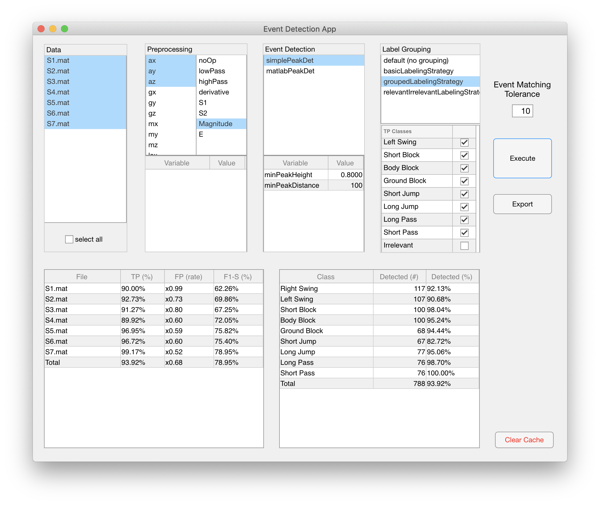
The Event Detection App can be used to compare the performance of different event detection algorithms. This includes the amount of relevant and irrelevant events detected for each recording session / file and the amount of events detected of each class.
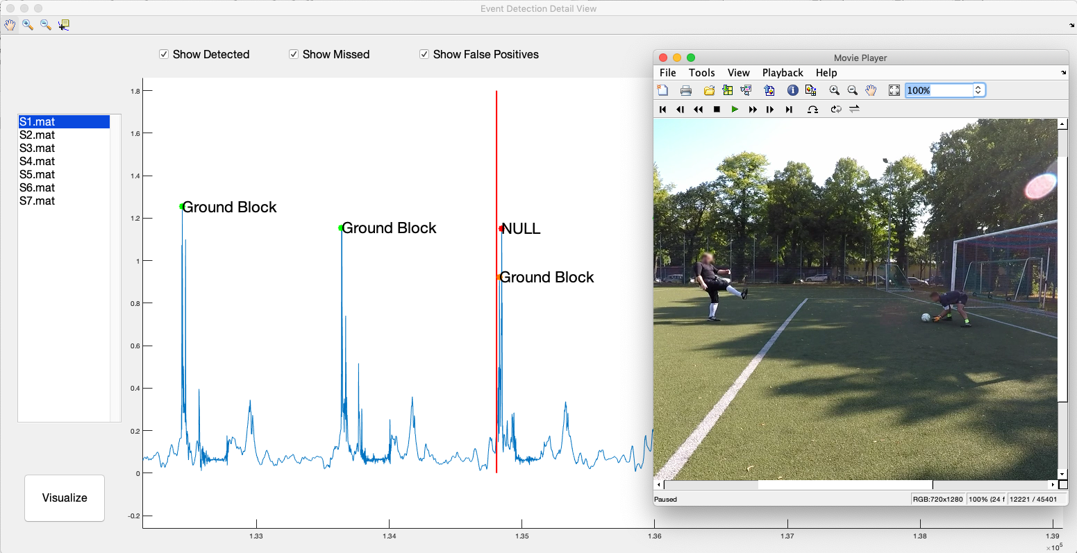
The Event Detection Detail View enables developers to gain insight into the performance of a particular event detection algorithm. Developers can zoom into the data and observe the detected and missed events together with the video.
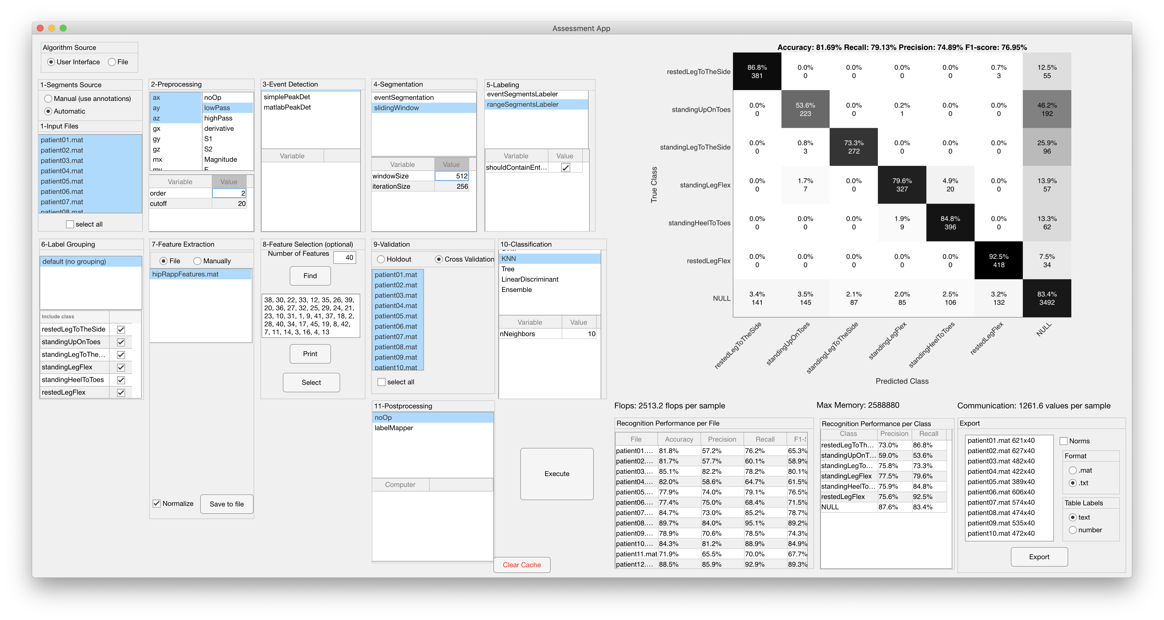
The development and assessement / evaluation of an activity recognition algorithm usually represents a large fraction of the effort to develop the entire application. The Assessment App enables developers to design algorithms by selecting reusable components at each stage of the activity recognition chain and to assess their performance. The recognition performance metrics provided by this tool are:
- Accuracy
- Precision
- Recall
- Confusion Matrix
and the computational performance metrics are:
- Flops: Number of floating point operations performed by the algorithm for the input data set
- Memory: Amount of memory consumed by the algorithm (in bytes) for the input data set
- Communication: Amount of bytes generated by the last component in the recognition chain
The image below shows the configuration and classification results of an algorithm to detect and classify exercises performed by patients after a hip replacement surgery.
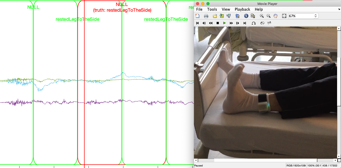
The Performance Asessment Detail View displays the classification results on top of the data and next to the corresponding video. Green overlays indicate correctly classified segments and red overlays indicate misclassified segments.
Note: Feature tables generated with a particular activity recognition algorithm can be exported to .txt formats to study the classification on other platforms such as python / tensorFlow and WEKA.
- The WDK loads data from a binary .mat file containing an instance of the DataFile class found in ./ARC/model directory. The Data Conversion App can load any file in CSV format and export it to the DataFile format. Place your CSV files in the ./data/rawdata/ directory.
- The labels used by the WDK should be listed in the .data/annotations/labels.txt file.
- Use the Data Annotation App to create a ground truth data set.
- (optional) Define a label grouping. A label grouping describes how labels annotated are mapped to groups used by the different Apps in the WDK. The following label grouping maps labels label1, label2 and label3 into Group1 and label4 and label5 to Group2.
#Group1
class1
class2
class3

#Group2
class4
class5
If no label grouping is defined, the WDK uses the defaultLabelingStrategy which maps each label to a class with the same name.
Note: Labels grouped in a label grouping should be defined in the './data/annotations/labels.txt' file.
Note: Label groupings should be placed in the './data/labeling/' directory.
Note: Labels should be mapped to a single group in a labeling strategy. Labels that are left ungrouped in a labeling strategy will be assigned to its own group automatically.
Most errors after installation are related to pathing issues. The paths used by the WDK are defined in the Constants.m file. Double-check the different paths in the Constants.m file exist in your file system.
Furthermore, errors identified by Matlab will be shown over the console:
'Error. Invalid annotation class'.
An annotation file in ./data/annotations/ contains an invalid label (i.e. a label which is not listed in the ./data/annotations/labels.txt file).
'Index in position 1 exceeds array bounds (must not exceed XXX).'
'Warning - FeatureSelector - every segment has same value. Feature selection might fail';
The current version of the FeatureSelector uses the mRMR algorithm to select the most relevant features. The mRMR algorithm will fail if every feature vector contains the same value for a particular feature.
The WDK has been developed based on Matlab's version 2018b. If Matlab crashes with these errors:
'Too many input arguments'
'Unrecognized property 'Scrollable' for class 'matlab.ui.Figure'
double-check that your are using Matlab 2018b or later.
Note: The data in the './data/rawData' directory should be consistent. You will get errors if different files have different amount of columns.
Note: Double-check that the './data/annotations/' directory contains an annotation file for each data file in './data/rawdata/'.
Note: A common error happens due to selecting incompatible computer nodes. As the WDK does not do type-checking on the computers selected, the first computer that received incompatible data will crash. If Matlab produces an error message with 'Computer.ExecuteChain' in its stack-trace, it is most likely due to an incompatible set of computers being used. In this case, double-check the input and output types of each computer.
- the feature selection feature in the WDK uses the mRMR library for feature selection. If you get an error 'estpab function not found', then you need to:
cd libraries/mRMR_0.9/mi/
mex -setup C++
makeosmex
- Matlab tutorial on Activity Recognition for wearables: https://github.com/avenix/ARC-Tutorial/
- Andreas Bulling's tutorial on Activity Recognition: https://dl.acm.org/citation.cfm?id=2499621
- Peak detection algorithms by Palshikar
- mRMR feature selection by Peng
- Nick Gillian's Gesture Recognition Toolki
Applications developed with the WDK:
My name is Juan Haladjian. I developed the Wearables Development Toolkit as part of my post-doc at the Technical University of Munich. Feel free to contact me with questions or feature requests. The project is under an MIT license. You are welcome to use the WDK, extend it and redistribute it for any purpose, as long as you give credit for it by copying the LICENSE.txt file to any copy of this software.
Email: haladjia@in.tum.de
Website: http://in.tum.de/~haladjia


