- Introduction
- Hardware
- Instruments
- Technologies
- Neural Network
- Model
- Tomidius
- Bibliography
- Developers
Tomidius consists of a system for real-time classification of cherry tomatoes. The application is able to distinguish intact tomatoes from those that have cuts or imperfections on the surface, based on the video streaming obtained from a webcam. The basic idea of the project is to create a stand alone system to be integrated into the assembly line of a fruit and vegetable company, which allows a quick classification of raw materials based on their appearance
Hardware components are:
- Raspberry Pi 3 Model B, a single board computer with Raspbian 9 installed on it;
- Logitech C920 HD Pro, a Full HD (1080p) USB webcam;
- Intel Neural Compute Stick 2 (NCS2), a Visual Processing Unit (VPU) that communicates with Raspberry trough USB;
In particular, the NCS2 module acts as an autonomous artificial intelligence accelerator, allowing greater speed of development and ease of release of solutions that exploit AI and Machine Learning technologies. It is used to have additional computing power during the inference phase.
Colaboratory is a cloud based Jupyter Notebook provided by Google. It therefore offers a Python development environment, complete with libraries such as TensorFlow, Keras, Matplotib, Numpy, etc ..., which runs on a remote virtual machine.
We have chosen to use this tool, instead of configuring a local environment, since it has guaranteed us greater simplicity of development and better performance, in terms of timing, during the training of the model, as there is the possibility of exploiting the hardware acceleration of a GPU or TPU provided by the Google machine.
It is the official toolkit provided by Intel necessary for the development of Computer Vision applications that must exploit NCS2 to make inference. In particular, it offered us the tools necessary to convert the model, from the Tensorflow model to the IR model readable by NCS2, and the drivers needed to communicate with this device.
It is an open source Google library that facilitates the development and deployment of Machine Learning applications. It offers various levels of abstraction so that you can decide on the most useful one as needed. It supports various programming languages, so as to adapt to the context of use. It also provides several useful services for production environments that need scalability and high levels of performance.
It is a high-level API written in Python that exploits the functionality of various libraries, including TensorFlow, allowing you to create and train models, greatly simplifying the programmer's work. Keras is strongly oriented towards experimentation, in fact it sees its main objective in the rapid development of models with good performances.
We used Keras, with Tensorflow backend, to build our convolutional network.
Python Object Oriented high-level language was used for development. Version 3.6 was used (as recommended by all documentation) for better integration with the various frameworks and toolkits.
It is an open source library that offers the programmer the possibility to communicate easily with video devices such as webcams, various computer vision algorithms and image processing. In this application, it is used to pre-process the image captured by the webcam, send every single frame to NCS2 to make the prediction and return the results through intuitive graphics.
A neural network is a network composed of at least an input layer, an intermediate layer (hidden) and an output layer, where a layer is a set of nodes (called neurons) belonging to the same level. Each neuron of a hidden layer contains an activation function that is applied to the input value received to obtain the output value returned by that neuron.
This function has the task of introducing nonlinearity into the model (for example the ReLU function).
Tomidius uses a convolutional neural network to classify the cherry tomato.
To make image classification, it is now common practice to build models based on the Convolutional Neural Network (CNN). A CNN is a neural network that takes an image as input and during training "learns" its characteristics, with the aim of inferring, at a later time, which object is contained in the new images that are placed at the input. We see below how a CNN is structured in detail.
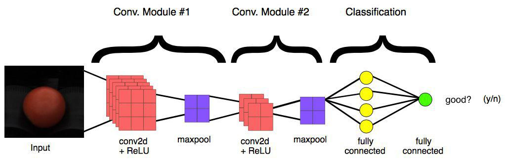
As just mentioned, CNN receives as input a three-dimensional matrix where the sizes of the first two dimensions correspond to the width and height, in pixels, of the image. The size of the third dimension is 3 (corresponding to the 3 color channels of an image: red, green and blue). A CNN has at least one convolution module composed of the Convolution + ReLU + MaxPooling layers and at least one Fully Connected layer (layer in which each node is connected with each node of the previous layer) preceding the Output layer. Now let's see how each of these layers works.
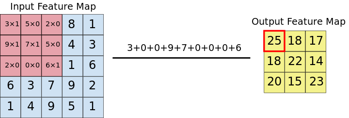
The convolution extracts blocks of the input matrix (called input feature map) and applies filters (of the same size as the extracted block) to calculate a new matrix (called output feature map) that can have different measures from the three-dimensional input matrix.
Convolution is defined by two parameters:
- Size of the input matrix block to be extracted (typically 3x3 or 5x5 pixel blocks are extracted);
- Depth of the new output matrix, which corresponds to the number of filters that are applied to the input matrix;
During the convolution, the entire input matrix is scrolled both horizontally and vertically, one pixel at a time, extracting from time to time the matrix block to which to apply the filter.
For each pair (piece of matrix - filter), CNN multiplies element by element and then adds all the elements of the resulting matrix to obtain a single value. Each resulting value composes an element of the output feature map:

During CNN training, it "learns" the optimal values of the filter matrices that show that they extract the significant characteristics (textures, edges, shapes) of the input images. All the tool of the number of filters that are applied (which determines the depth of the three-dimensional output matrix) increases the number of filters that CNN is able to recognize. However, typically, we try to choose the minimum number of filters to extract the required characteristics, since the training time increases the whole instrument by the number of filters applied.
Following each convolution, CNN applies a Rectified Linear Unit (ReLU) to each element of the matrix coming from the convolution, so as to introduce non-linearity in the model. ReLU function:
After ReLU, MaxPooling takes place, an operation with which CNN resizes the convolution matrix, reducing the size of the first two dimensions (width and height), while preserving the most critical information. MaxPooling operates in a similar way to convolution, scrolling the matrix that is presented to it at the input and extracting pieces of a set size. For each piece of extracted matrix, the maximum value among all its elements is the output value that makes up the single element of the new output matrix. All other values are therefore discarded. It is an operation characterized by two parameters:
- Max pooling filter size (typically 2x2 pixels);
- Step: the distance, in pixels, with which the filter "moves" on the input matrix between one sampling and another. Unlike what happens with convolution, in which the filters slide pixel by pixel over the whole matrix, in max pooling the step determines how many pixels you move (horizontally and vertically) during the extractions;
At the end of a convolutional network there are one or more layers called Fully Connected. When two layers are fully connected, each node in the first layer is connected with each node in the second layer. Their task is to make the classification based on the characteristics extracted from the previous convolution modules. Typically, the last fully connected layer contains a softmax as an activation function, which outputs a probability of 0 to 1 for each classification label that the model is trying to predict.
In our case, the output layer is a fully connected layer composed of a single neuron that has a sigmoid as its activation function, which outputs the percentage of goodness of the cherry tomato (a number from 0 to 1).
An example of a simple convolutional network could be the one in the following figure:
The dataset available to us was provided by Unitec SpA, it contains 557 images of cherry tomatoes in good condition and 520 images of cherry tomatoes in poor condition, for a total of 1077 images (actually quite small dataset, which greatly influenced the choice on the network adopted and model training techniques). The dataset was organized as follows:
- Training set: 75% of the data (808 images);
- Validation set: 25% of the data (269 images);
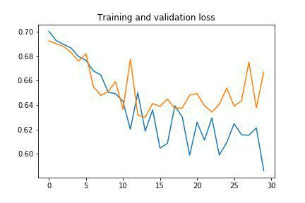
The first approach was to create and train a custom from scratch CNN. Multiple combinations have been tried, in order to achieve the highest possible accuracy, while reducing the loss. The final configuration of the network consists of:
- Three Convolution modules, with an incremental number of 3x3 filters (16, 32, 64);
- A Flatten layer, to reduce the matrix coming out of the convolution modules to a one-dimensional tensor;
- A Fully Connected layer consisting of 512 nodes with ReLU activation function;
- A Dropout layer, which during training randomly removes units from the neural network. It is a technique used to mitigate the overfitting of the model to the dataset;
- The output layer with a single node, on which a sigmoidal activation function acts which decrees the prediction value. In this last layer, this activation function is necessary since the problem is binary in the solution: a cherry tomato can be good or not. The sigmoidal function responds exactly to this need, in fact its output is a number in the range [0.1], which describes the probability that the image belongs to that of a good cherry tomato;
The chosen loss function is the binary cross-entropy (or log loss), useful for checking the loss for binary problems; in fact, if the predicted value is close to the label supplied, the loss value will be close to 0, otherwise it will be very high.
The optimization algorithm chosen is RMSprop, because it automates the learning rate adjustment process (similar to the Adagrad and Adam algorithms).
Below are the graphs of the (fairly poor) results of the training.
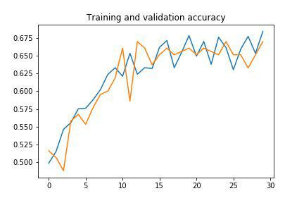
Given the low performance of the custom network, a transfer learning approach was attempted, which basically ensures better performance; in fact, this procedure involves the use of a network already trained on a very large dataset, which saves a lot of time on training and provides greater accuracy.
MobileNet is a consolidated network built by Google and widely used for image classification, so it was chosen as the starting network.
We have chosen to use the version of the model trained with the ImageNet dataset, because it is an extremely large and complete image dataset.
We proceeded as follows:
- The MobileNet network is part of the Keras library integrated in TensorFlow, therefore its import into the project is very simple;
- The final layer has been removed from the MobileNet network, the layer that makes the final decision for the model, so as to be able to add the decision layers useful to our needs;
- We then added to the bottom of the network:
- A Flatten layer to make the output of the one-dimensional MobileNet network;
- Two Fully Connected layers of 512 and 1024 nodes with ReLU activation function;
- A final 1 node fully connected layer with sigmoidal activation function, which provides the final result of the inference;
- Initially the freezing (see Model) of the MobileNet network was chosen, avoiding to train also its layers, thus having a static network unable to learn, but this entailed barely acceptable performances;
- Subsequently, the layers were left free to learn and this greatly increased the performance of the network;
- The choice to leave the layers free to learn has influenced the choice of the optimization algorithm (the Stochastic Gradient Descent) and of the learning rate index, deliberately kept low;
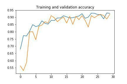
At this point the training of the model has given excellent results.
Below are the graphs of the results (this time extremely good) of the training.

Here is a summary table with the most common metrics to evaluate the goodness of the predictions of a neural network. In particular:
- Loss: it is an indicator of the error made by the model in making a prediction on a data item, therefore the lower the value of this parameter, the better the predictions of the model (Loss = 0 indicates a perfect model). Validation Loss is the same parameter calculated on the data of the validation set;
- Accuracy: represents the number of correct predictions compared to the total number of predictions, high percentages indicate a better ability of the model to predict correctly (Accuracy = 100% indicates a perfect model). Validation Accuracy is the same parameter calculated on the data of the validation set;
- Precision: indicates how many of all the images that were predicted as good were actually images of good cherry tomatoes; higher values indicate greater correctness of predictions;
- Recall: indicates how many of all the images that must be predicted as images of good cherry tomatoes have been correctly predicted; higher values indicate greater correctness of predictions;
Note: Precision and Recall have been calculated on the validation set.
There is a significant improvement in all areas of the network with transfer learning from MobileNet compared to the custom network.
| Loss | Accuracy | Validation Loss | Validation Accuracy | Precision | Recall | |
|---|---|---|---|---|---|---|
| MobileNet | 0,181 | 92,7% | 0,232 | 88,3% | 0,936 | 0,936 |
| Custom | 0,605 | 67,2% | 0,650 | 65,1% | 0,618 | 0,846 |
When the model has achieved sufficient performance and after carrying out several tests with images unrelated to the dataset, it has gone to the export phase, so as to be able to obtain a model with which to carry out assessments locally, no longer depending on the environment generated with Colaboratory. In order to obtain a model on which to make inferences it is necessary to go through a freezing phase.
This phase acts directly on the weights associated with the connections of the neural network, i.e. those values that are learned during the training phase and that during the evaluation cause the activation of certain neurons, in response to the particular characteristics of the data given in input to the network.
During the training phase these weights are variable, i.e. their value can be changed between different periods or different workouts.
The freezing phase involves fixing the weights, making them no longer modifiable, but fixing them as constant and immutable values, in order to have a stable model, with consistent performance between different executions. As a result of the freeze, a descriptive file of the model with .pb extension is produced, all-inclusive of the structure of the network and the weights associated with the trained model.
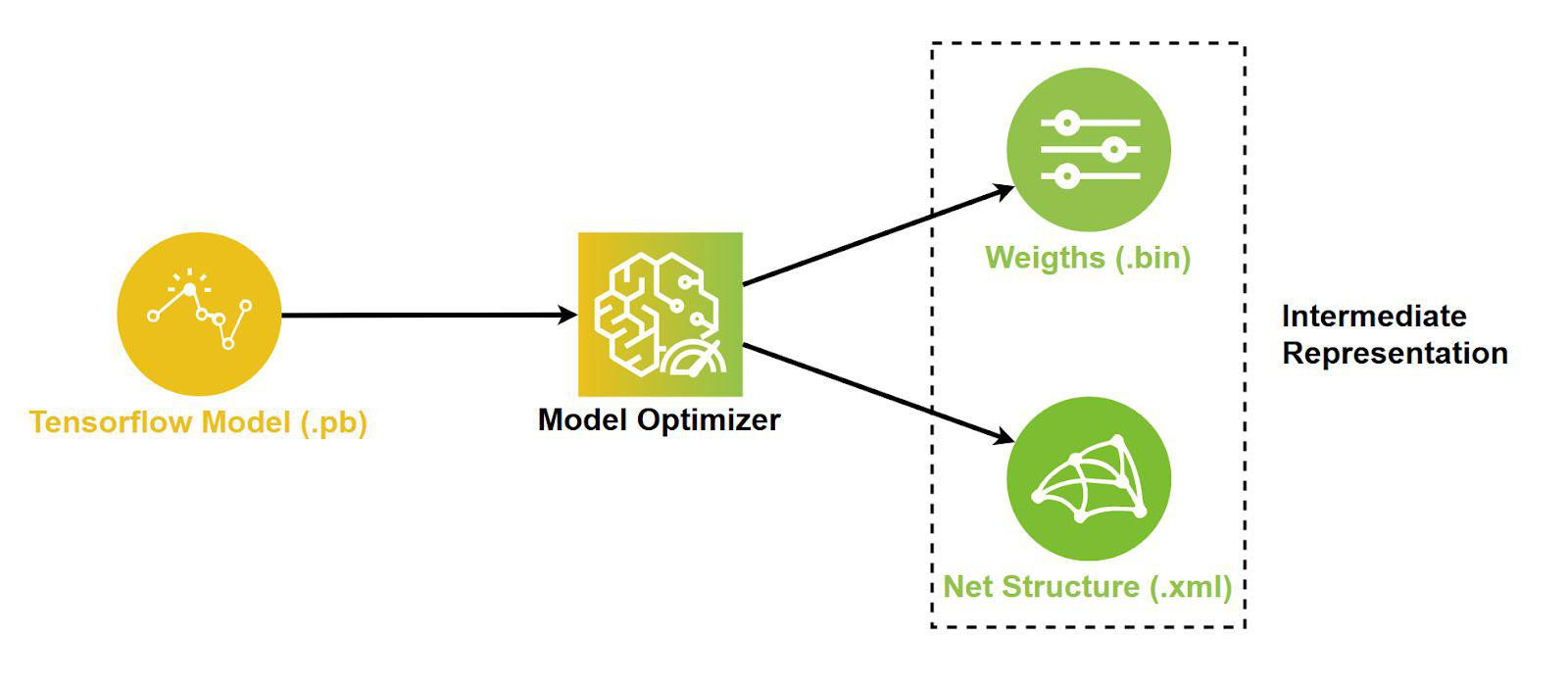
Once brought locally, the model in .pb format must undergo a conversion in order to be interpreted by NCS2. This is requested regardless of the type of model considered, in fact conversion is required whether it is a Caffe, Kaldi, Tensorflow model (as in our case), etc.
The conversion phase is carried out using the Model Optimizer offered by the OpenVINO toolkit.
The Model Optimizer is a cross-platform command-line tool that facilitates the transition between the training environment and the execution environment, also allows you to perform static analysis of the model and ensures optimal execution on the target devices.
In our case it was necessary to specify to the Model Optimizer the type of input and the data type of the network:
- Input Shape: (1,224,224.3);
- Data Type: FP16;
A 16 bit floating point precision has been set via the data type (the only one supported by NCS2). While the input shape describes to the Model Optimizer the shape of the inputs that will be passed to the network.
In our case these inputs provide batches of unit size (the network computes only one image at a time) and data of size 224x224x3, where 224x224 is the size of the images while 3 represents the associated RGB channels.
At the end of the conversion phase, the Model Optimizer returns two files:
- <model_name> .xml: describes the internal structure, therefore all the layers, of the network;
- <model_name> .bin: contains all the weights, calculated during the training of the net;
These two files represent the Intermediate Representation (IR) of the model, which is the only format with which it is possible to perform inference operations on the NCS2 module, using a custom model.
The system consists of a Raspberry Pi 3 Model B to which the NCS2 module and the Logitech webcam are connected via USB.
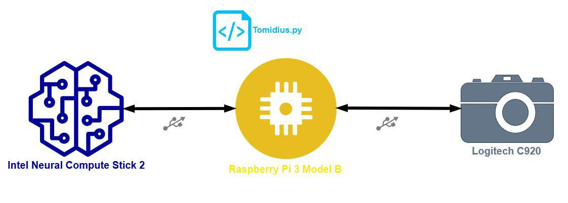
The tomidius.py script is run on the Raspberry, which starts the system. The application receives the images captured by the webcam and examines them frame by frame.
Each frame extrapolated from the flow is first preprocessed, in particular a square of size 224x224 is cut out where the cherry tomato will be framed. The user will be helped to correctly position the tomato through a window showing the streaming input from the webcam, on which the box that delimits the area of interest is drawn.
At this point, each frame is processed, i.e. a prediction operation is performed on the image thanks to the network model (properly converted).
The result of the prediction is a number between the range [0.1], if the value tends to 0 then the cherry tomato is classified as faulty, otherwise (if it tends to 1) it is classified as good.
The result of this analysis phase is shown to the user through the same window mentioned above, through an intuitive graphic that describes the picked up cherry tomato. Alternatively, from the command line it is possible to view the real value (in percentage form) that the network provides at the end of the prediction, so as to have a better understanding of the actual classification capabilities of the model.
The system, in order to work at its best, requires that the cherry tomato be taken on a black background and in low light conditions. These limitations derive from the way in which the images were collected for the dataset, which are not very bright and without any variety in the backgrounds. However, it was not considered a problem, as due to the nature and objectives of the project, it can easily be assumed that in production the application operates in controlled and standardized conditions.
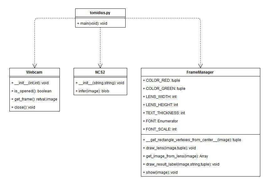
Below is the class diagram to assist in reading the code. Note that the tomidius.py file is not a real class, but it is a script that acts as an entry point for the application.