Losses in image classification task

Image classification is a dominant task in machine learning. There are lots of competitions for this task. Both good architectures and augmentation techniques are essential, but an appropriate loss is crucial nowadays.

For example, almost all top teams in Kaggle Protein Classification challenge used diverse losses for training their convolutional neural networks. In this story, we’ll investigate what losses apply in which case.

Focal loss

If there is a rare class in your dataset, its contribution to a summary loss is slight. To cope with this problem, the authors of the article https://arxiv.org/abs/1708.02002 suggest applying an additional scale factor which reduces losses of those samples the model is sure of. Hard mining is provoking a classifier to focus on the most difficult cases which are samples of our rare class.

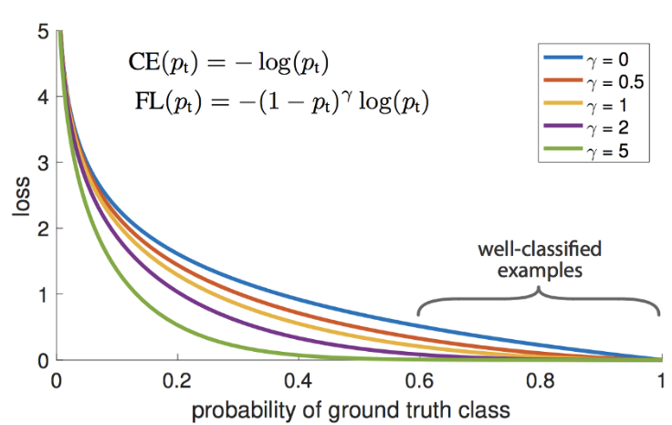
$$ p_{\mathrm{t}}=\left{\begin{array}{ll}{p} & {\text { if } y=1} \ {1-p} & {\text { otherwise }}\end{array}\right. $$

Gamma controls decreasing speed for easy cases. If it’s close to 1 and the model is insecure, Focal Loss acts as a standard Softmax loss function.

Center loss

Softmax loss only encourages the separation of labels, leaving the discriminative power of features aside. There is a so-called center loss approach, as described in the article https://arxiv.org/abs/1707.07391. In addition to CE loss, center loss includes the distance from the sample to a center of the sample’s class.

$$ L=L_{s}+\lambda L_{c} $$

$L_s$ denotes the Softmax loss, $L_c$ denotes the center loss. $\lambda$ is a scaling factor.

$$ L_{c}=\frac{1}{2} \sum_{i=1}^{m}\left|x_{i}-c_{y_{i}}\right|_{2}^{2} $$

Where $L_c$ denotes the center loss $m$ denotes the number of training samples in a min-batch. $x_i \in \mathbb{R}^{d}$ denotes the $i$-th training sample. $y_i$ denotes the label of $i$. $c_{y_i} \in \mathbb{R}^{d}$ denotes the $y_i$-th class center of deep features. $d$ is the feature dimension.

These two approaches give the following results:

Contrastive center loss

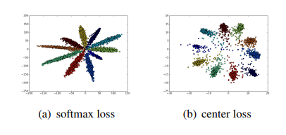
The center loss only stimulates intra-class compactness. This does not consider inter-class separability. Moreover, as long as the center loss concerns only the distances within a single class, there is a risk that the class centers will be fixed. In order to eliminate these disadvantages, a penalty for small distances between the classes was suggested.

$$ L_{c t-c}=\frac{1}{2} \sum_{i=1}^{m} \frac{\left|x_{i}-c_{y_{i}}\right|{2}^{2}}{\left(\sum{j=1, j \neq y_{i}}^{k}\left|x_{i}-c_{j}\right|_{2}^{2}\right)+\delta} $$

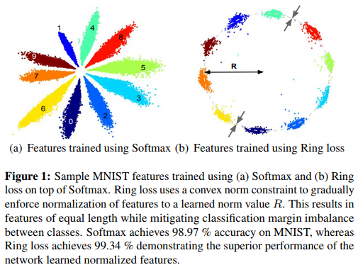
Where $L_{c t-c}$ denotes the contrastive-center loss. $m$ denotes the number of training samples in a min-batch. $x_{i} \in R_{d}$ de- notes the $i$ th training sample with dimension $d$ is the fea- ture dimension. $y_{i}$ denotes the label of $x_{i} . c_{y_{i}} \in R_{d}$ denotes the $y_{i}$ th class center of deep features with dimension $d . k$ de- notes the number of class. $\delta$ is a constant used for preventing the denominator equal to $0 .$ In our experiments, we set $\delta=1$ by default.

Ring loss

Instead of learning centroids directly, there is a mechanism with a few parameters. In the article ‘Ring loss’, the authors justified that the maximum angular margin is reached when the norm of feature vectors is the same. Thus, stimulating samples to have the same norm in a feature space, we:

Increase the margin for better classification.
Apply the native normalization technique.

$$ L_{R}=\frac{\lambda}{2 m} \sum_{i=1}^{m}\left(\left|\mathcal{F}\left(\mathbf{x}{i}\right)\right|{2}-R\right)^{2} $$ where $\mathcal{F}\left(\mathbf{x}{i}\right)$ is the deep network feature for the sample $\mathbf{x}{i}$.

Visualizing features in 2D space we see the ring.

ArcFace loss

Softmax loss is formulated as:

$$ L_{1}=-\frac{1}{N} \sum_{i=1}^{N} \log \frac{e^{W_{y_{i}}^{T} x_{i}+b_{y_{i}}}}{\sum_{j=1}^{n} e^{W_{j}^{T} x_{i}+b_{j}}} $$

where $x_i \in \mathbb{R}^{d}$ denotes the deep feature of the $i$-th sample, belonging to the $y_i$-th class. The embedding feature dimension $d$ is set to 512 in this paper following [38, 46, 18, 37]. $W_j \in \mathbb{R}^{d}$ denotes the $j$-th column of the weight $w \in \mathbb{R}^{d \times n}$ and $b_{j} \in \mathbb{R}^{n}$ is the bias term. The batch size and the class number are $N$ and $n$, respectively.

$$ W_{j}^{T} x_{i}=\left|W_{j}\right|\left|x_{i}\right| \cos \theta_{j} $$

They also fix the feature’s vector norm to 1 and scale norm of feature sample to $s$. Now our predictions depend only on the angle between the feature vector and weight vector.

$$ L_{2}=-\frac{1}{N} \sum_{i=1}^{N} \log \frac{e^{s \cos \theta_{y_{i}}}}{e^{s \cos \theta_{y_{i}}}+\sum_{j=1, j \neq y_{i}}^{n} e^{s \cos \theta_{j}}} $$

In order to increase intra-class compactness and improve inter-class discrepancy, an angular margin is added to a cosine of $\theta_{y_i}$.

$$ L_{3}=-\frac{1}{N} \sum_{i=1}^{N} \log \frac{e^{s\left(\cos \left(\theta_{y_{i}}+m\right)\right)}}{e^{s\left(\cos \left(\theta_{y_{i}}+m\right)\right)}+\sum_{j=1, j \neq y_{i}}^{n} e^{s \cos \theta_{j}}} $$

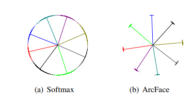
For a comparison, let’s look at the picture above! There are 8 identities there in 2D space. Each identity has its own color. Dots present a sample and lines refer to the center direction for each identity. We see identity points are close to their center and far from other identities. Moreover, the angular distances between each center are equal. These facts prove the authors’ method works.

SphereFace and CosFace losses

These losses are very close to ArcFace. Instead of performing an additive margin, in SphereFace a multiplication factor is used:

$$ L_{\mathrm{ang}}=\frac{1}{N} \sum_{i}-\log \left(\frac{e^{\left|\boldsymbol{x}{i}\right| \cos \left(m \theta{y_{i}, i}\right)}}{\left.e^{\left|\boldsymbol{x}{i}\right| \cos \left(m \theta{y_{i}}, i\right)}+\sum_{j \neq y_{i}} e^{\left|\boldsymbol{x}{i}\right| \cos \left(\theta{j, i}\right)}\right)}\right) $$

Or CosFace relies on a cosine margin:

$$ L_{l m c}=\frac{1}{N} \sum_{i}-\log \frac{e^{s\left(\cos \left(\theta_{y_{i}, i}\right)-m\right)}}{e^{s\left(\cos \left(\theta_{y_{i}}, i\right)-m\right)}+\sum_{j \neq y_{i}} e^{s \cos \left(\theta_{j, i}\right)}} $$

LGM loss

Authors of the article https://arxiv.org/pdf/1803.02988 rely on Bayes’ theorem to solve a classification task.

They introduce LGM loss as the sum of classification and likelihood losses. Lambda is a real value playing the role of the scaling factor.

$$ \mathcal{L}{G M}=\mathcal{L}{c l s}+\lambda \mathcal{L}_{l k d} $$

Classification loss is formulated as a usual cross entropy loss, but probabilities are replaced by the posterior distribution:

$$ p\left(x_{i} | z_{i}\right)=\mathcal{N}\left(x_{i} ; \mu_{z_{i}}, \Sigma_{z_{i}}\right) $$

$$ \begin{aligned} \mathcal{L}{c l s} &=-\frac{1}{N} \sum{i=1}^{N} \sum_{k=1}^{K} \mathbb{1}\left(z_{i}=k\right) \log p\left(k | x_{i}\right) \ &=-\frac{1}{N} \sum_{i=1}^{N} \log \frac{\mathcal{N}\left(x_{i} ; \mu_{z_{i}}, \Sigma_{z_{i}}\right) p\left(z_{i}\right)}{\sum_{k=1}^{K} \mathcal{N}\left(x_{i} ; \mu_{k}, \Sigma_{k}\right) p(k)} \end{aligned} $$

The classification part acts as a discriminative one. But there is an additional likelihood part in the article:

$$ \mathcal{L}{l k d}=-\sum{i=1}^{N} \log \mathcal{N}\left(x_{i} ; \mu_{z_{i}}, \Sigma_{z_{i}}\right) $$

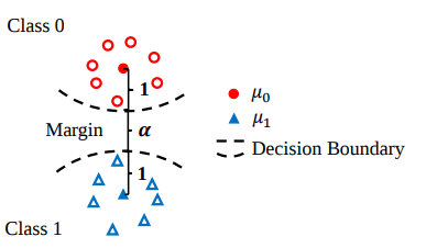
This term forces features $x_i$ to be sampled from the normal distribution with appropriate mean and covariance matrix.

In the picture one can see samples which have the normal distribution in 2D space.

origin 中文翻译

FLHonker/Losses-in-image-classification-task