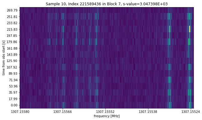
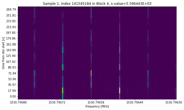
Finding small slices of data like this:

From huge amounts of data (10s of Gigabytes every 5 minutes), and then figuring out their type and origin. (Radios? Satillites? Microwave oven across the hall? Aliens?)
(Skipping generic text about how important SETI is)
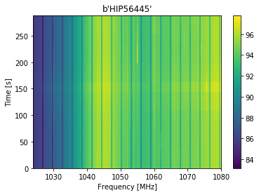
A lot of the data that Breakthrough Listen is collecting is in the form of dynamic spectrums, which we call waterfalls. They look like this:
The x axis is Frequency, the y axis is time, and each point has a power reading representing how much energy is coming from that frequency at that timestep.
If you look at the part where the frequency is about 1060 Mhz, you can see a thin bright line in the plot, that's a signal, and if you look closely, there are many more bright lines in the plot, which are of course all signals picked up by the telescope.
The goal of this project is building a database of "seen" signals and constructing a pipeline for picking out signals from every observation and using dimensionality reduction to match them to seen ones. If we find a signal that's unseen before from any of our observations, that means we've found ET! (or a bug)
In our observations, there will often be broadband signals (for example at t=150s in the plot above). These signals come from high energy FRI that spill over all the channels. For this project, we are only interested in narrowband signals because we are assuming an extraterrestial transmitter would choose to transmit in narrower bands.
To remove the broadband signals, we normalize the average power of each spectrum (timestep) to 1. Because these files are very large: about 16 GB each, we use Dask to process the file in parallel, speeding up the computation process and removing the need to read the whole file into memory.
The resulting plot is mostly the same as the original, but without the broadband features. In the example below, there was a broadband "burst" in the 8th spectrum. After processing, the "burst" was removed.
| Original | Broadband Features Removed |
|---|---|
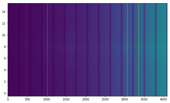 |
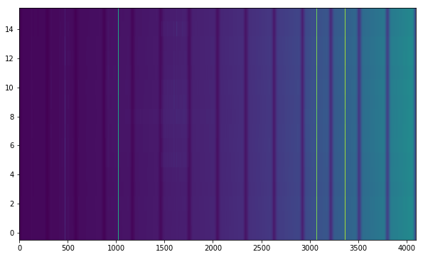 |
The result is stored as 22 npy blocks, each containing 16 spectrums in 14 channels (the original file is 16 spectrums by 308 channels).
[describe bandpass]
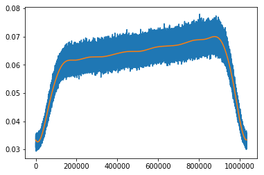
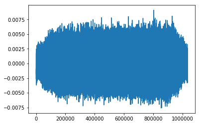
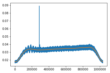
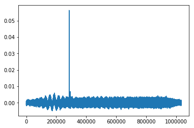
To remove the bandpass, we use spline lines to fit each channel to obtain a model of the bandpass of that channel. By using splines, we are able to fit the bandpass without fitting the more significant signals. This is illustrated below.
| Original & Spline Fit | Original minus Spline Fit |
|---|---|
 |
 |
 |
 |
The upper two plots shows a channel containing mostly noise, but the bandpass creates a plateau-like shape whose edges may interfere with our gaussianity tests. After fitting the data with a spline line (in orange), we can take the residuals of the fit and retrieve data which is close to gaussian noise.
In channels with narrowband features, the plateau shape of the bandpass is also removed, but the narrowband signal remains unchanged relative to the noise.
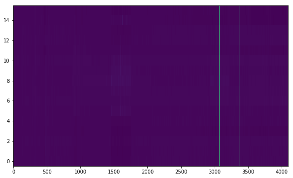
Performing this operation on a block of data generates the plot below:
For comparision, here is the same section with the bandpass:
And here is the original data, with broadband features and bandpass:
We attempt to take narrow "stamps" covering 0.0005 Mhz each. These "stamps" are essentially slices of the data that are 16 by 200 elements. Based on a priori knowledge, we can assume that the background noise received by the telescope is gaussian noise. Therefore, if a stamp deviates from a gaussian distribution, or has excess energy, it is likely to contain a signal.
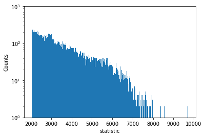
We use scipy.stats.normaltest, which implements D’Agostino and Pearson’s omnibus test for normality to calculate a statistic and the corresponding p-value. A higher statistic, or a lower p-value means a larger deviation from gaussian noise. Because the calculated p-values are often too small to be represented with floating point numbers, we use the statistic for filtering. For now, we use a threshold of 2048 because it yields a reasonable amount of samples after filtering.
Plotting a histogram of the statistic value of sample stamps from the data confirms our intuition that the number of samples in ranges of equal length decreases as the statistic value increases. This means that as samples deviate further from gaussian, the likelihood of that sample being seen decreases.
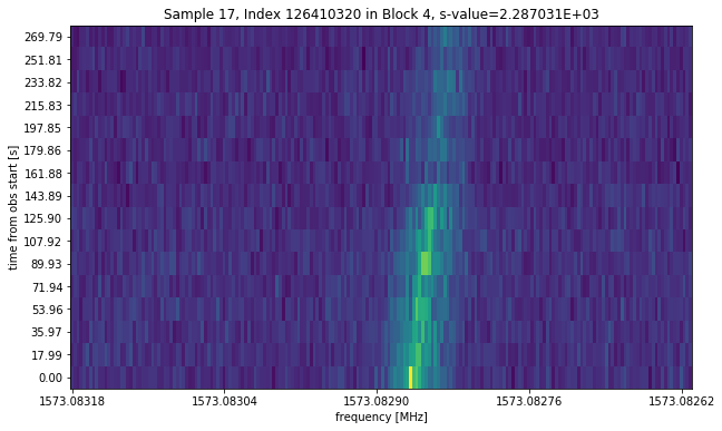
We also show some sample stamps with differing statistic values to illustrate the relationship between the statistic and the detected signal. Below are three sample stamps with increasing statistic values.
The first sample with a statistic of around 2000 depicts a single drifting signal that is in the same range of intensity as the background noise (as the noise is clearly visible). The second sample with higher statistic value shows multiple narrowband signals that are relatively stronger, as the background is darker compared to the first sample. While the last sample shows the background as completely dark, meaning that the shown signals have much larger intensity.


