Cost of train journeys

To install this package, download this repository and run the following from the root directory of the repo:

# # If you have not previously installed poetry before...
# type the following for osx/linux/bashonwindows:
# curl -sSL https://raw.githubusercontent.com/python-poetry/poetry/master/get-poetry.py | python -
# or type the following if you're on Windows:
# (Invoke-WebRequest -Uri https://raw.githubusercontent.com/python-poetry/poetry/master/get-poetry.py -UseBasicParsing).Content | python -
# See https://python-poetry.org/docs/ for details on installation
poetry install

To open a Python session with all the dependencies you can run the following:

poetry shell
poetry run python
# From the Python shell, load the package to test it's installed:
import railfares

You can get the stations reachable with the specified budget from the specified starting station by running the following code:


starting_station = 'newcastle'

budget = 10

df = data_parsing.get_isocost_stations(starting_station, budget)

Useful links

Train stations are referred to using a range of different systems in the data set. Other than the official station name, each station usually has a common name, a CRS code, an NLC code, and a TIPLOC code. A relatively comprehensive list of these systems is available here.

Data on the location of train stations with coordinates is available, amongst other sources, as part of the National Public Transport Access Nodes (NaPTAN) data set.

For developing and debugging, it can be useful to check the fares of specific journeys manually. A great resource to do this is the BR FARES website which gives access to all flows and fares between pairs of stations for all ticket types (select ``Expert Mode'' when querying).

Tutorial

This is a brief tutorial on how to use this package. The tutorial is also avaiable as a separate script in tutorial.py.

The functions of this package are implemented in data_parsing.py. Any other script is analysing the rail fares data using the basic functions implemented in the package.

NOTE: the mapping functionalities currently use the free-tier services of MapBox to retrieve the map tiles via my account API token. Please create maps in moderation, or replace the token with a different one!

To start with, let's import all the relevant packages we will need in this tutorial:

import railfares.data_parsing as data_parsing
import pandas as pd
import geopandas as gpd
from folium.plugins import MarkerCluster
from matplotlib.colors import rgb2hex
import folium

As a first example, we will calculate the list of stations you can reach with a given budget from a starting station. In the following, we refer to this as an isocost (in analogy with isochrones). Note, however, that this is not strictly speaking going to be a list of stations all reachable with the same budget (as the name isocost would imply), but rather all stations reachable with the given maximum budget. This means that most stations will actually be reachable with a lower budget.

We start by specifying the name of a starting station, for instance Exeter St Davids:

starting_station = 'exeter st davids'

We then specify the maximum budget we want to use for the calculation:

budget = 10

Again, as noted above, this is a maximum fare, not the exact fare. Next, we calculate the isocost:

isocost = data_parsing.get_isocost_stations(starting_station, budget)

After running this, the isocost variable contains a Pandas dataframe with all the stations that can be reached from the starting station with the given budget. The returned data frame contains the names of all the stations, and the corresponding fare. It also contains more technical information on the route, station code names, etc.

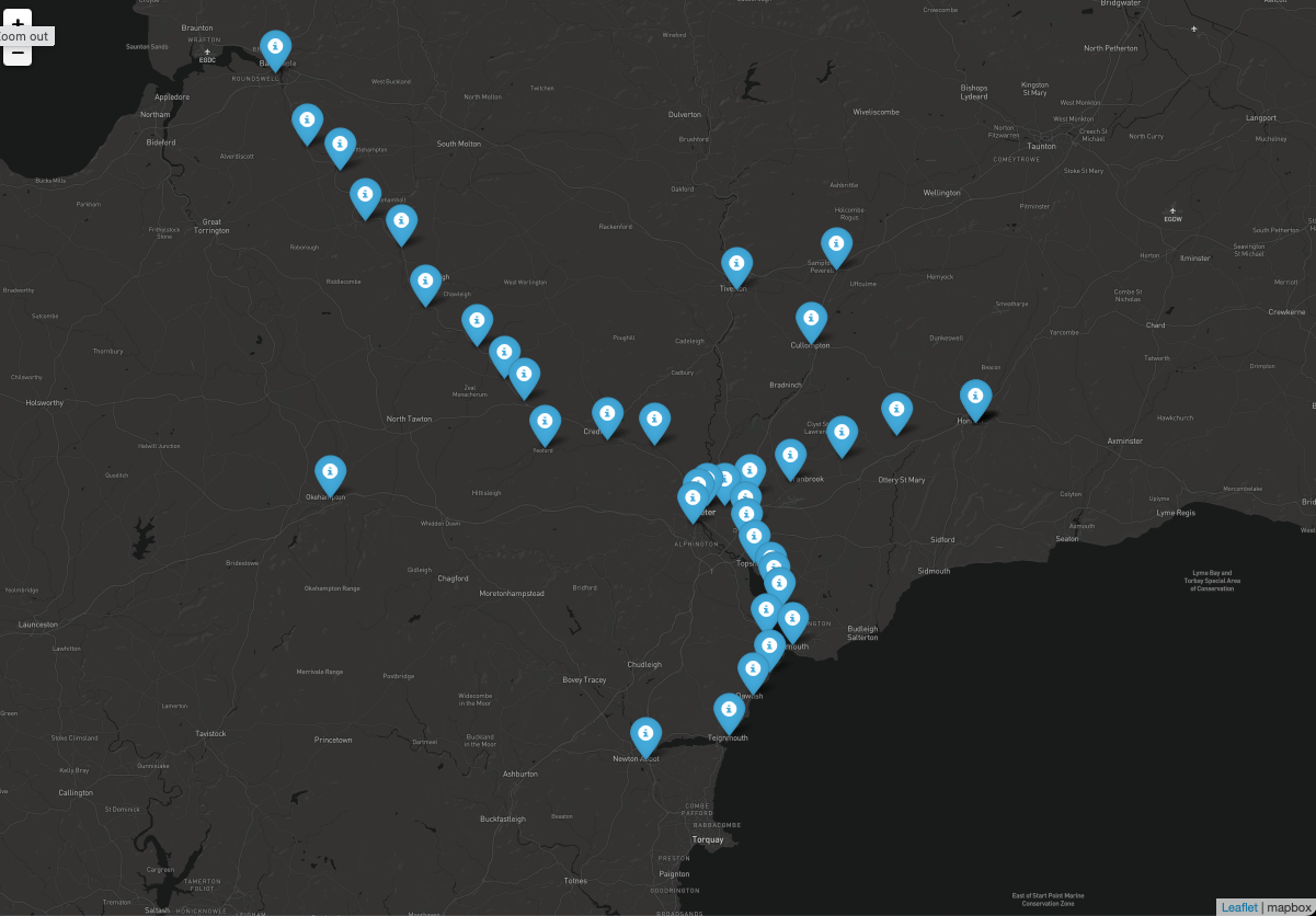
You can then create a map of the stations that can be reached. The following outputs to file an interactive html map:

#first, set the file path and name (use .html as file extension)
file_path_name = 'USE_PATH_AND_FILE_NAME_TO_OUTPUT'

#then create and output the map
data_parsing.plot_isocost_stations(starting_station, isocost, file_path_name)

Which should look something like this (note that, however, this map was created using MapBox tiles, for which you need an API token; the tutorial uses tiles from Stamen):

You can also use the pre-calculated OD matrix to retrieve the cost of reaching any station from the starting station. NOTE: this section requires to have the OD matrix file

First, read the OD file. This is a large file so will take some time to read and use a significant amount of memory:

od_list = pd.read_csv('od_minimum_cost_matrix.csv', low_memory = False)

Next, select the entries corresponding to journeys starting at the starting station NOTE: the starting station string is converted to upper as in the OD matrix this is how the station names typically appear. This is for the tutorial purpose only, as in general it is more accurate to work with CRS or TIPLOC codes which are unique and do not depend on abbreviation of station names.

station_od = od_list[od_list['Origin station name'] == starting_station.upper()].copy()

This next section of code creates a map to plot the cost of reaching any station from the starting station defined above.

In order to create a map with a good colour scheme, we set a maximum price of 300 GBP; however, in practice this is usually not exceeded for journeys considered here, but might need to be changed if considering a different type of journeys.

max_price = 300
step = 10
bins = list(range(0, max_price + step, step))
n_bins = max_price / step


labels = []
colour_step = 240/n_bins

r = 240
g = 240
b= 240

for i in range(0, int(n_bins), 1):
    
    labels.append(rgb2hex([r/255, (g)/255, (b)/255]))
    g = g - colour_step
    b = b - colour_step
    
station_od['marker_colour'] = pd.cut(station_od['fare'], bins = bins,
                                    labels =labels)

station_od['Destination station name'] = station_od['Destination station name'].str.rstrip()
station_od['popupText'] = ['Starting station: ' + starting_station + ',<br> Destination station: ' + row['Destination station name'].lower() + ',<br> Fare: £' + str(row['fare']).ljust(4,'0') for idx, row in station_od.iterrows()]

naptan_gdf = data_parsing.get_naptan_data()
naptan_gdf = naptan_gdf.to_crs(epsg = 4326)

station_gdf = data_parsing.get_station_location(tiploc = True)
station_gdf = station_gdf.to_crs(epsg = 4326)

stations = gpd.GeoDataFrame(naptan_gdf.merge(station_gdf, left_on = 'TIPLOC', right_on = 'tiploc_code', how = 'left').drop(columns = ['geometry_y', 'Easting', 'Northing'], axis = 1).rename(columns = {'geometry_x': 'geometry'}))

station_od_gdf = stations.merge(station_od, left_on = 'CRS Code', right_on = 'destination_crs')

od_list_min = station_od_gdf.loc[station_od_gdf.groupby(['Destination station name'])['fare'].idxmin()]

cost_map = folium.Map(location = [station_gdf.dissolve().centroid[0].coords[0][1],station_gdf.dissolve().centroid[0].coords[0][0]], 
                      tiles = "https://api.mapbox.com/styles/v1/mapbox/dark-v10/tiles/{z}/{x}/{y}?access_token=pk.eyJ1IjoiZmVkZWJvdHRhIiwiYSI6ImNsNnZzZmx1bDA0aXozYnA5NHNxc2oxYm4ifQ.NH-kHQqlCLP3OVnx5ygJlQ",
                      attr='mapbox', zoom_start = 7)
# svg_style = '<style>svg {background-color: white;}</style>'

# colormap.get_root().header.add_child(folium.Element(svg_style))
# cost_map.add_child(colormap)

marker_cluster = MarkerCluster(name = "Train stations").add_to(cost_map)

od_list_min = od_list_min.to_crs(epsg = 4326)

for idx, row in od_list_min.iterrows():
    
    
    folium.CircleMarker([row["geometry"].y, row['geometry'].x],
                  icon=folium.Icon(color = '#000000', icon_color=row['marker_colour']),
                  fill = True, fill_color = row['marker_colour'], color = '#000000', fill_opacity = 0.75, radius = 8, weight = 1,
                  popup = row['popupText']).add_to(cost_map)

#use this variable to specify the path and file name(with .html extension) where the map should be saved
file_path_name = ''
cost_map.save(file_path_name)

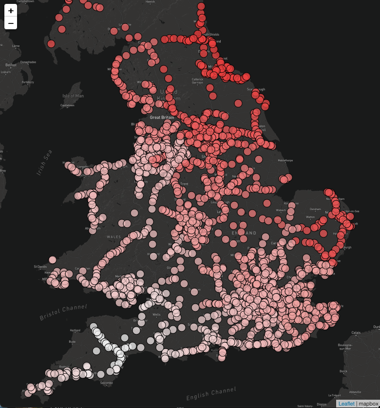
The resulting map should look something like this (as for the above map, this was generated using tiles from MapBox):

where darker shades of red correspond to a higher fare.

Output data

The data realesed as part of this package can be found in the Releases. There are a number of files available, and here we provide a description of their structure (for more information on how the data set was generated, see paper):

od_minimum_cost_matrix.csv: this file contains the miminum fare between pairs of stations, as described in the paper. The file has one entry per row, and the following columns:

Column label	Description
Destination station name	The common name of the destination station.
nlc_code	The National Location Code (NLC) for the destination station. NLC are codes associated to each train station.
origin_code	This is the code representing the flow origin. It can either be a station NLC or a cluster NLC.
destination_code	This is the code representing the flow destination. It can either be a station NLC or a cluster NLC.
route_code	The route code.
end_date	The date until which this flow fare is valid.
start_date	The date from which this flow fare is valid.
toc	The fare code of the Train Operating Company (TOC) setting the fare.
flow_id	The unique identifier of this flow.
cluster_id	The cluster NLC of the starting station.
fare	The fare of this flow, in GBP (£).
Origin station name	The commone name of the starting station.
origin_crs	The Computer Reservation System (CRS) code of the starting station.
destination_crs	The CRS code of the destination station.

number_hospitals_xx_pounds.csv: this series of files (where xx is a number) contains the number of hospitals that can be reached from any station for a budget of £xx. The file has one entry per row, and the following columns:

Column label Description

origin_crs The CRS code of the origin station.

Count The number of hospitals that can be reached from the origin station with the budget.

Note: the files number_large_employment_centres_xx_pounds.csv, number_medium_employment_centres_xx_pounds.csv and number_town_centres_xx_pounds.csv all have this structure too. See paper for a description of how they were generated.

Column label	Description
origin_crs	The CRS code of the origin station.
Count	The number of hospitals that can be reached from the origin station with the budget.

stations_stats_xx_pounds.csv: this series of files (where xx is a number) contains some statistics of how far you can travel from a given station with a given budget of xxx. The file has one entry per row, and the following columns:

Column label	Description
Station CRS	The CRS code of the starting station
Number	The number of stations you can travel to from the starting station with the budget.
Max distance	The maximum distance to a station, in metres, you can travel to from the starting station with the budget.
Mean distance	The mean distance, in metres, you can travel to from the starting station with the budget.
Median distance	The median distance, in metres, you can travel to from the starting station with the budget.

stations_pairwise_distances.csv: this file contains the distance, in metres, between each pair of stations. The file has one entry per row, and the following columns:

Column label	Description
First CRS	The CRS code of the first station in the pair.
Second CRS	The CRS code of the second station in the pair.
Distance	The distance between the two stations.

stations_stats_and_pop_xx_pounds.csv: this series of files (where xx is a number) is experimental and should be ignored for now.
mean_price_change.csv: this file is experimental and should be ignored for now.

FedericoBotta/railfares

Cost of train journeys

Useful links

Tutorial

Output data