Fast Density-Based Clustering Validation (DBCV) implementation for Python, with support for parallel and dynamically-adjustable high precision computation.
Fully compatible with the original MATLAB implementation available in https://github.com/pajaskowiak/dbcv/.
NOTE: See below for instructions on how to ensure equivalent results to the MATLAB implementation if strictly required in your application.
python -m pip install "git+https://github.com/FelSiq/DBCV"

|
import dbcv
import sklearn.datasets

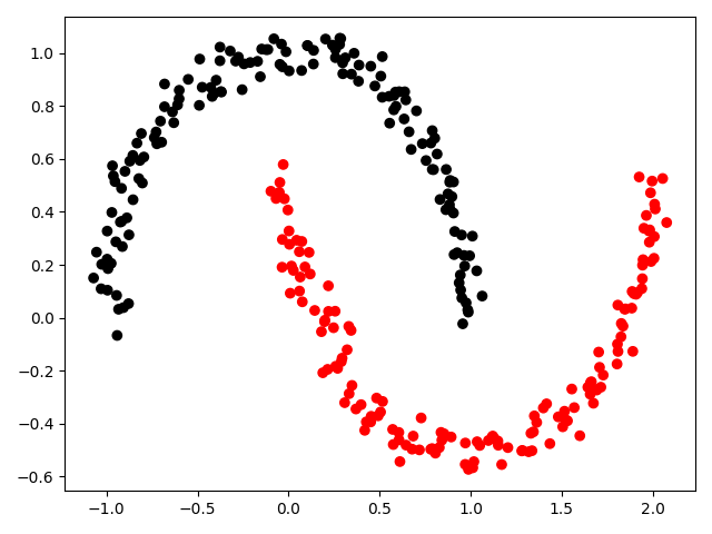
X, y = sklearn.datasets.make_moons(n_samples=300, noise=0.05, random_state=1782)

score = dbcv.dbcv(X, y)
print(score)
# 0.8545358723390613 |
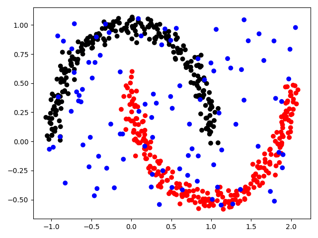
The DBCV metric naturally supports clustering configurations where some instances have not been clustered and are considered noise. By default, all instances with the cluster ID of -1 are considered noise (you can replace this ID with a custom value), as demonstrated in the example below.
You can use the dbcv.dbcv(..., n_processes=n) argument to specify the number of parallel processes during computations. The default value of n_processes is "auto", which is equivalent to 1 for datasets with 500 or fewer instances, and 4 for datasets with more than 500 instances.
import dbcv
import sklearn.datasets

X, y = sklearn.datasets.make_moons(n_samples=300, noise=0.05, random_state=1782)

score = dbcv.dbcv(X, y, n_processes=2)
print(score)
# 0.8545358723390613If you are facing underflow issues and need more precision bits, you can dynamically adjust how many are available by enabling dbcv.dbcv(..., enable_dynamic_precision=True). The number of precision bits available is controlled by dbcv.dbcv(..., enable_dynamic_precision=True, bits_of_precision=n).
import dbcv
import sklearn.datasets

X, y = sklearn.datasets.make_moons(n_samples=300, noise=0.05, random_state=1782)

score = dbcv.dbcv(X, y, enable_dynamic_precision=True, bits_of_precision=512)
print(score)
# 0.8545358723390613
Note that enabling this option makes the DBCV calculation much slower than the plain numpy/scipy version. However, this option may be necessary for computing DBCV in high dimensions, since density calculations easily underflow under that circumstance. The table below displays runtimes from computing DBCV on an dataset of shape (10,000, 784) twenty times in a row for variable amount of precision bits and for dynamic precision disabled.
| Bits | Runtime mean ± std (slowdown w.r.t. 'Off') |
|---|---|
| Off (64 bits) | 8.7808 ± 0.0475 |
| 64 | 42.8156 ± 0.2801 (+3.88x) |
| 128 | 45.3012 ± 0.0959 (+4.16x) |
| 256 | 49.8338 ± 0.2369 (+4.68x) |
| 512 | 58.2917 ± 0.1223 (+5.64x) |
| 1024 | 80.1517 ± 0.2222 (+8.13x) |
This package is designed to be fully compatible with the original MATLAB implementation (see references for URL). However, a few convenient changes have been made to the default setup:
- The default noise cluster ID (label) is -1 instead of 0 (as in the MATLAB implementation). This change was made to ensure easier compatibility with popular packages like scikit-learn, which adopts the convention of labeling noise instances as -1. You can adjust the noise cluster ID using the argument
dbcv(..., noise_id=0). - The default Minimum Spanning Tree (MST) algorithm used is Scipy's Kruskal's MST implementation. The original MATLAB implementation uses a variant of Prim's MST algorithm. This package also provides a direct translation to Python of the MATLAB implementation. If you require strictly equivalent results to the original implementation, you can change the MST algorithm by setting
dbcv(..., use_original_mst_implementation=True). Note that the original implementation is expected to be slower than Scipy's implementation and tends to generate hub nodes more frequently (i.e., resulting trees are not equivalent). Experimental results showing differences between both implementations can be checked in this issue.
Similar to the original MATLAB implementation, this package uses the squared Euclidean distance as the default distance metric. You can modify the metric by using dbcv(..., metric="metric_name"). All metrics implemented in Scipy are supported.
The following execution should be equivalent to the original source code execution:
import dbcv
X, y = ...
score = dbcv.dbcv(X, y, metric="sqeuclidean", noise_id=0, use_original_mst_implementation=True)
For reference, the Table below exhibits a comparison between the results estimated by this Python implementation (using both MST algorithm implementations) and the original MATLAB code. The datasets are available in the MATLAB GitHub repository.
| Dataset | Python (Scipy's Kruskal's) | Python (Translated MST algorithm) | MATLAB |
|---|---|---|---|
dataset_1.txt |
0.8566 | 0.8576 | 0.8576 |
dataset_2.txt |
0.5405 | 0.8103 | 0.8103 |
dataset_3.txt |
0.6308 | 0.6319 | 0.6319 |
dataset_4.txt |
0.8456 | 0.8688 | 0.8688 |
- Moulavi, Davoud & Andretta Jaskowiak, Pablo & Campello, Ricardo & Zimek, Arthur & Sander, Joerg. (2014). Density-Based Clustering Validation. 10.1137/1.9781611973440.96.
- https://github.com/pajaskowiak/dbcv/
MIT.

