The paper has been accepted for publication at the 27th European Conference on Artificial Intelligence (ECAI'24). The full version (preprint) is available here.
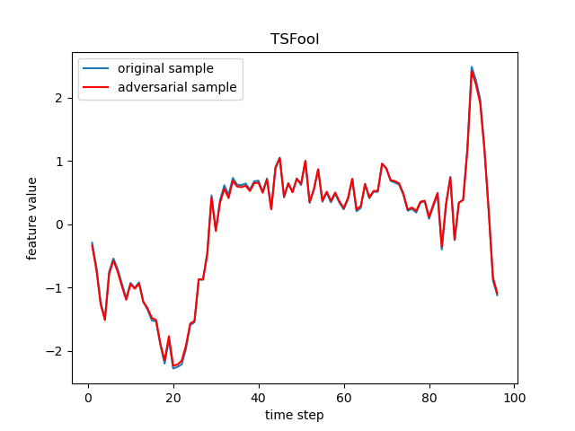
TSFool is a multi-objective gray-box attack method to craft highly-imperceptible adversarial samples for RNN-based time series classification. The TSFool method in this repository is built for univariate time series data, and an extended version called Multi-TSFool for multivariate time series data can be found here.
- The pre-trained RNN classifiers used in our experiments are available here.
- The adversarial sets generated by TSFool are available here.
- The detailed experimental setup can be found here.
$ git clone https://github.com/FlaAI/TSFool.git
$ cd TSFool
$ python
  >>> # load your target model and dataset #
  >>> from main import TSFool
>>> adv_X, target_Y, target_X = TSFool(model, X, Y)adv_X, target_Y, target_X = TSFool(model, X, Y, K=2, T=30, F=0.1, eps=0.01, N=20, P=0.9, C=1, target=-1, details=False)Given a target time series dataset (X, Y) and the corresponding RNN classifier model, TSFool can automatically capture potential vulnerable samples to craft highly-imperceptible adversarial perturbation, and finally output a generated adversarial set adv_X, as well as the captured original samples target_X and their labels target_Y.
Empirically, we provide default values of all the hyper-parameters used, while of course you can adjust them according to specific practices to achieve better performance. Below is some information that may be found useful:
The hyper-parameters K, T, F are introduced for the establishment of a representation model used in TSFool named intervalized weighted finite automaton (i-WFA). Specifically, K, T come from the original WFA model, so for the adjustment of their value, we recommend the paper "Decision-guided weighted automata extraction from recurrent neural networks" where WFA is proposed for more details. On the other hand, F is introduced by us to determine the size of domain interval for the input abstraction in the establishment of i-WFA. The larger the value of F, the finer-grained the interval, which leads to the more precise input abstraction but weaker generalization for unseen data.
The hyper-parameters eps, N, P, C are used to control the crafting of adversarial samples, respectively for the perturbation amount, the number of adversarial samples generated from every single pair of vulnerable sample and target sample, the possibility of a random masking noise used, and the number of target sample matched for every specific vulnerable sample. Notice that the larger the value of P, the less the randomness of masking noise, which means the higher attack success rate but the more similar adversarial samples generated from the same pair of vulnerable sample and target sample. The TSFool support both targeted and untargeted attack, and the target is provided for specifying your target label.
If you are interested in the detailed attack process of TSFool, please value details to be True to print more run-time information.
- model (nn.Module): the target rnn classifier.
- X (numpy.array): time series sample (sample_amount, time_step, feature_dim).
- Y (numpy.array): label (sample_amount, ).
- K (int): >=1, hyper-parameter of build_WFA(), denotes the number of K-top prediction scores to be considered.
- T (int): >=1, hyper-parameter of build_WFA(), denotes the number of partitions of the prediction scores.
- F (float): (0, 1], hyper-parameter of build_WFA(), ensures that compared with the average distance between feature points, the grading size of tokens is micro enough.
- eps (float): (0, 0.1], hyper-parameter for perturbation, denotes the perturbation amount under the limitation of 'micro' (value 0.1 corresponds to the largest legal perturbation amount).
- N (int): >=1, hyper-parameter for perturbation, denotes the number of adversarial samples generated from a specific minimum positive sample.
- P (float): (0, 1], hyper-parameter for perturbation, denotes the possibility of the random mask.
- C (int): >=1, hyper-parameter for perturbation, denotes the number of minimum positive samples to be considered for each of the sensitive negative samples.
- target (int): [-1, max label], hyper-parameter for perturbation, -1 denotes untargeted attack, other values denote targeted attack with the corresponding label as the target.
- details (bool): if True, print the details of the attack process.
Based on manifold hypothesis, a possible explanation for the existence of adversarial samples is that the features of input data cannot always visually and semantically reflect the latent manifold, which makes it possible for the samples considered to be similar in features to have dramatically different latent manifolds. As a consequence, even a small perturbation in human eyes added to a correctly predicted sample may completely change the perception of NN to its latent manifold, and result in a significantly different prediction.
So if there is a representation model that can imitate the mechanism of a specific NN classifier to predict input data, but distinguish different inputs by their features in the original high-dimensional space just like a human, then it can be introduced to capture deeply embedded vulnerable samples whose features deviate from latent manifold, which can serve as an effective guide for the crafting of perturbation in adversarial attack.
This idea can be especially useful when white-box knowledge like model gradients are not fully and directly available, and its advantage in the imperceptibility can be significantly revealed by the attack on some types of data that are sensitive to perturbation in particular (as the RNN model + time series data we focus on here).
The UCR Time Series Classification Archive: https://www.cs.ucr.edu/~eamonn/time_series_data_2018/
We select the 10 experimental datasets following the UCR briefing document strictly to make sure there is no cherry-picking. To be specific, the claims for the data are:
- 30
$\leq$ Train Size$\leq$ 1000, since the pre-training of RNN classifiers is not a main part of our approach and is not expected to spend too much time, while a too-small training set may make the model learning unnecessarily challenging, and a too-big training set is more likely to be time-consuming respectively; - Test Size
$\leq$ 4000, since all the attack methods are based on the test set to craft adversarial samples and we expect to compare them efficiently; and - class numbers
$\leq$ 5 and time step length$\leq$ 150, since they represent the scale of the original problem which we also would like to reduce due to the same reason as above.
Note that all the claims are proposed just for a compromise between general significance and experimental efficiency of our evaluation (since hopefully this would be suitable for reporting in a technology paper), instead of an inherent limitation of TSFool. Just as the "best practice" suggested by the UCR briefing document, hopefully we will gradually test and publish the results of TSFool attack on all the rest of the UCR datasets in the future.
| ID | Type | Name | Train | Test | Class | Length |
|---|---|---|---|---|---|---|
| CBF | Simulated | CBF | 30 | 900 | 3 | 128 |
| DPOAG | Image | DistalPhalanxOutlineAgeGroup | 400 | 139 | 3 | 80 |
| DPOC | Image | DistalPhalanxOutlineCorrect | 600 | 276 | 2 | 80 |
| ECG200 | ECG | ECG200 | 100 | 100 | 2 | 96 |
| GP | Motion | GunPoint | 50 | 150 | 2 | 150 |
| IPD | Sensor | ItalyPowerDemand | 67 | 1029 | 2 | 24 |
| MPOAG | Image | MiddlePhalanxOutlineAgeGroup | 400 | 154 | 3 | 80 |
| MPOC | Image | MiddlePhalanxOutlineCorrect | 600 | 291 | 2 | 80 |
| PPOAG | Image | ProximalPhalanxOutlineAgeGroup | 400 | 205 | 3 | 80 |
| PPOC | Image | ProximalPhalanxOutlineCorrect | 600 | 291 | 2 | 80 |
Important Update: We have reconstructed the implementation of the benchmarks by moving from the Torchattacks (Paper, Resource) to the Adversarial Robustness Toolbox (ART) (Paper, Resource) because the latter seems more popular and powerful to support sufficient comparison in this task. Our great thanks to the contributors of both of the two public packages!
There are totally nine existing adversarial attacks adopted as benchmarks in our evaluation.
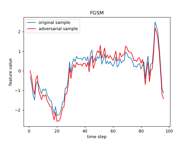
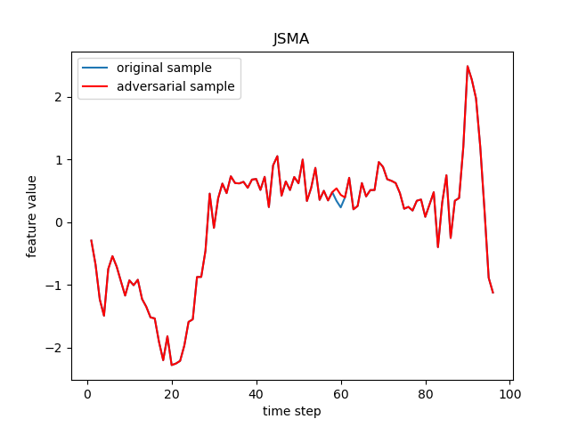
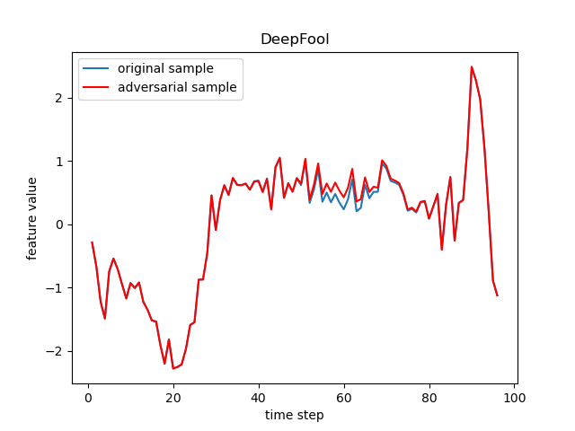
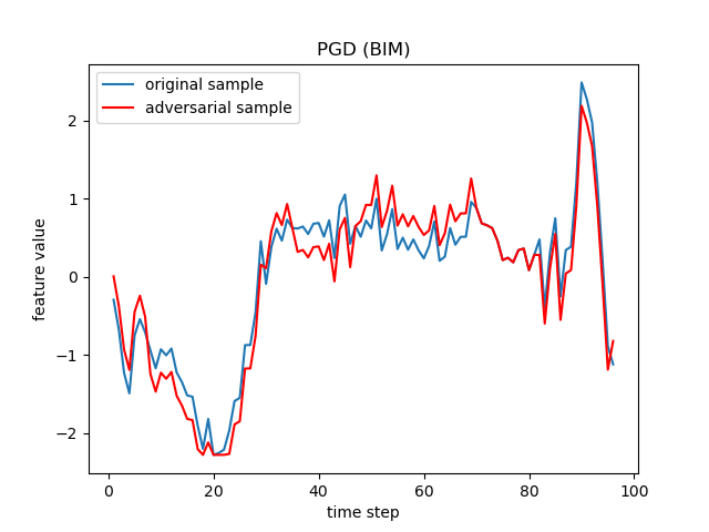
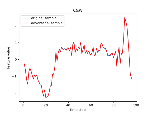
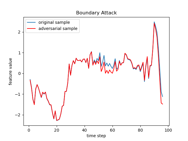
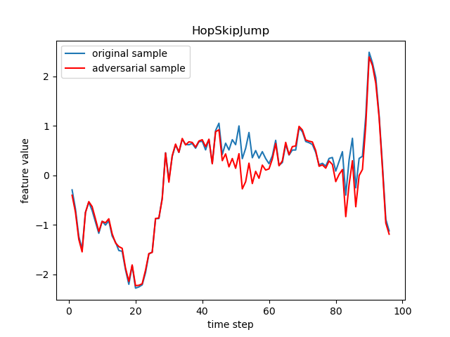
The FGSM, JSMA, DeepFool, PGD (sometimes referred to as BIM in deep learning), C&W, Auto-Attack, Boundary Attack and HopSkipJump are popular adversarial attack methods from basic to state-of-the-art ones, respectively from the following papers:
- FGSM: Explaining and harnessing adversarial examples.
- JSMA: The Limitations of Deep Learning in Adversarial Settings.
- DeepFool: DeepFool: A Simple and Accurate Method to Fool Deep Neural Networks.
- PGD: Towards Deep Learning Models Resistant to Adversarial Attacks.
- BIM: Adversarial Examples in the Physical World.
- C&W: Towards Evaluating the Robustness of Neural Networks.
- Auto-Attack: Reliable evaluation of adversarial robustness with an ensemble of diverse parameter-free attacks.
- Boundary Attack: Decision-Based Adversarial Attacks: Reliable Attacks Against Black-Box Machine Learning Models.
- HopSkipJump: HopSkipJumpAttack: A Query-Efficient Decision-Based Attack.
Our specific implementation of these attacks is as follows:
# Initialize PyTorchClassifier for ART
classifier = PyTorchClassifier(
    model=model,
    loss=nn.CrossEntropyLoss(),
    optimizer=torch.optim.Adam(model.parameters(), lr=LR),
    input_shape=(X.shape[1], X.shape[2]),
    nb_classes=CLASS_NUM,
    clip_values=(min_X_feature, max_X_feature),
    channels_first=False
)

# Define experimental attack methods by ART
fgsm = FastGradientMethod(classifier)
jsma = SaliencyMapMethod(classifier)
deepfool = DeepFool(classifier)
pgd = ProjectedGradientDescent(classifier)
cw = CarliniLInfMethod(classifier)
apgdce = AutoProjectedGradientDescent(classifier, loss_type='cross_entropy')
auto = AutoAttack(classifier, attacks=[pgd, apgdce, deepfool])
boundary = BoundaryAttack(classifier, targeted=False)
hsj = HopSkipJump(classifier, targeted=False)
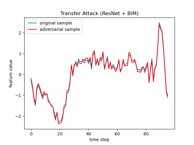
On the other hand, for the Transfer Attack, a public adversarial UCR set (generated by ResNet + BIM) is used:
