This project is part of the Udacity self-driving car nanodegree. I use a number of computer vision techniques to identify lane lines on a curving road in differing road conditions. Output videos of the work are stored here:
- ./output_images/output_project_video.mp4 "Project Video"
- ./output_images/output_challenge_video.mp4 "Challenge Video"
- Compute the camera calibration matrix and distortion coefficients given a set of chessboard images.
- Apply a distortion correction to raw images.
- Use color transforms, gradients, etc., to create a thresholded binary image.
- Apply a perspective transform to rectify binary image ("birds-eye view").
- Detect lane pixels and fit to find the lane boundary.
- Determine the curvature of the lane and vehicle position with respect to center.
- Warp the detected lane boundaries back onto the original image.
- Output visual display of the lane boundaries and numerical estimation of lane curvature and vehicle position.
- Real time lane detection for autonomous vehicles, Assidiq et. al.
- Saad Bedros, Hough Transform and Thresholding lecture, University of Minnesota
- Lane detection techniques review, Kaur and Kumar
- An Adaptive Method for Lane Marking Detection Based on HSI Color Model, Tran and Cho
- LANE CHANGE DETECTION AND TRACKING FOR A SAFE-LANE APPROACH IN REAL TIME VISION BASED NAVIGATION SYSTEMS, Somasundaram, Ramachandran, Kavitha
- A Robust Lane Detection and Departure Warning System, Mrinal Haloi and Dinesh Babu Jayagopi
- Steerable filters
- A layered approach to robust lane detection at night, Hayes and Pankati
- SHADOW DETECTION USING COLOR AND EDGE INFORMATION
- fillpoly example: https://www.programcreek.com/python/example/89415/cv2.fillPoly
- search around poly from coursework. I did it in y, and this is convenient in x
- extracting frames from video: https://stackoverflow.com/questions/33311153/python-extracting-and-saving-video-frames
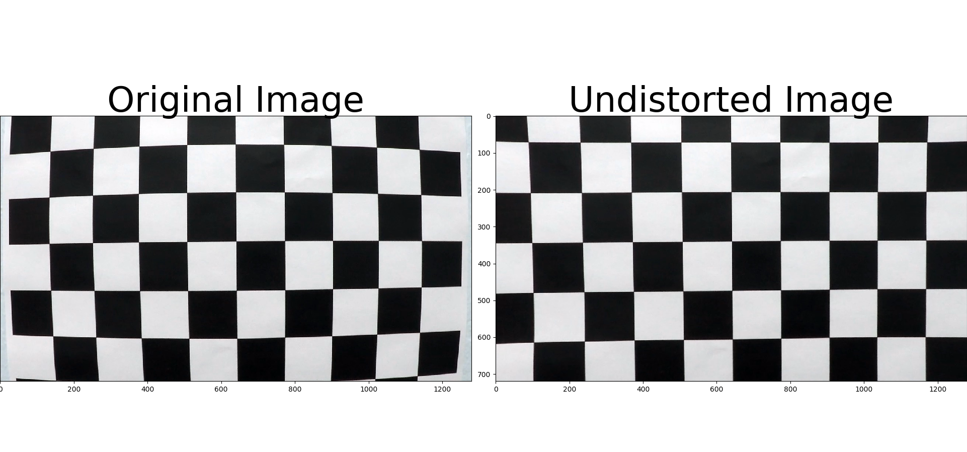
1. Briefly state how you computed the camera matrix and distortion coefficients. Provide an example of a distortion corrected calibration image.
The code for this step is contained in the first code cell of the IPython notebook located in "./examples/example.ipynb" (or in lines # through # of the file called some_file.py).
I start by preparing "object points", which will be the (x, y, z) coordinates of the chessboard corners in the world. Here I am assuming the chessboard is fixed on the (x, y) plane at z=0, such that the object points are the same for each calibration image. Thus, objp is just a replicated array of coordinates, and objpoints will be appended with a copy of it every time I successfully detect all chessboard corners in a test image. imgpoints will be appended with the (x, y) pixel position of each of the corners in the image plane with each successful chessboard detection.
I then used the output objpoints and imgpoints to compute the camera calibration and distortion coefficients using the cv2.calibrateCamera() function. I applied this distortion correction to the test image using the cv2.undistort() function and obtained this result:
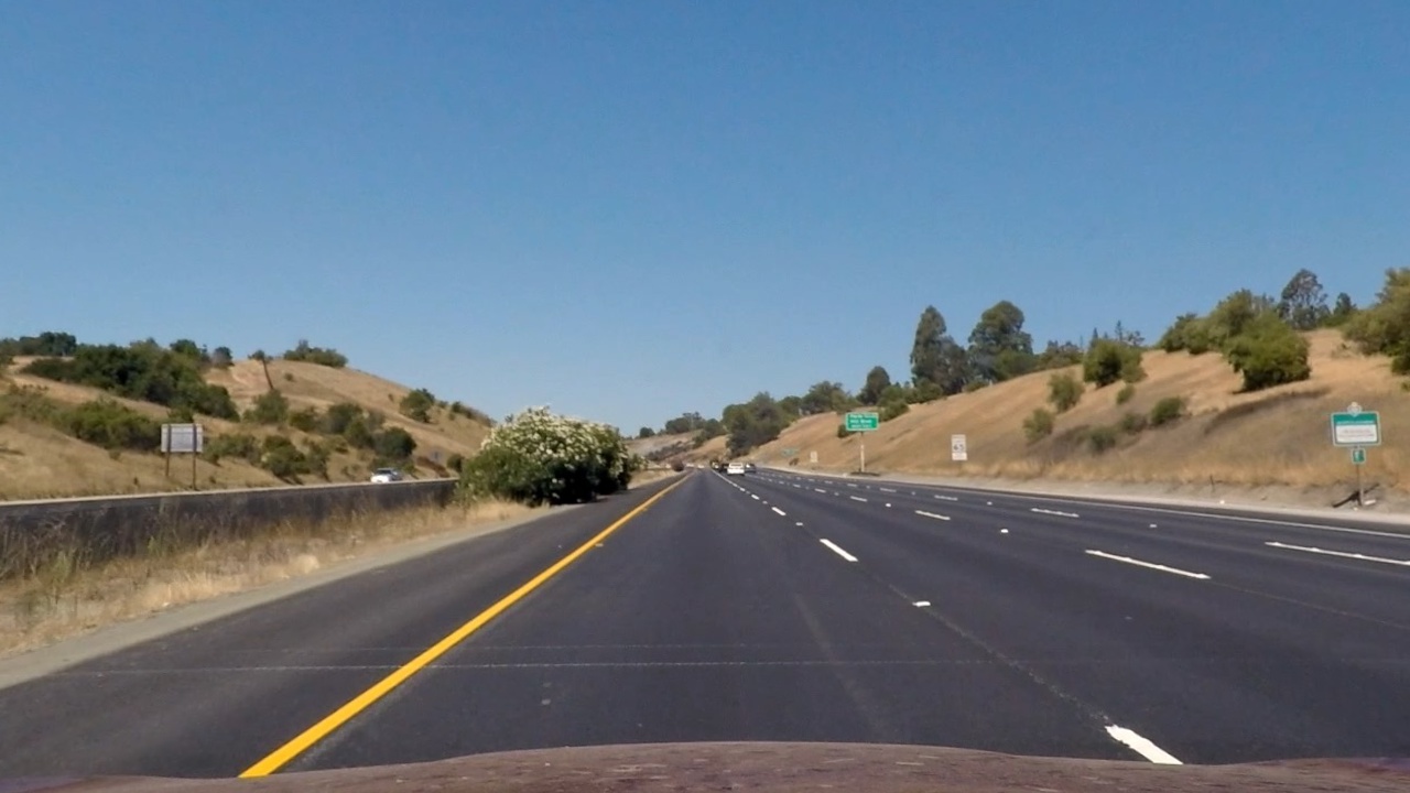
I use a helper function called cal_undistort to apply the distortion matrix to an input image. To demonstrate this step, I will describe how I apply the distortion correction to one of the test images like this one:

2. Describe how (and identify where in your code) you used color transforms, gradients or other methods to create a thresholded binary image. Provide an example of a binary image result.
I used a combination of color and gradient thresholds to generate a binary image (thresholding steps at lines 17 through 56 the pipeline cell of my Jupyter workbook called Advanced Lane Finding.ipynb. Here's an example of my output for this step. 
For edge detection, I use the red channel instead of the grayscale. It does a much better job of picking up the lane lines in varying color conditions, especially on bright colored roads. I look for vertical gradients with high magnitude that are picked up by the SobelX operator. This picks up lines in shadows as well.
For white lines, I combine L with (S OR Gradient R). Both S and Gradient R pick up white lines well. However Gradeint R does a much better job of picking up lines that are far away. S seems to be limited in its distance. Both of these bring in a lot of noise. ANDing them with high L gets rid of the noise.
For yellow lines, I combine S with Low H. It works well, but has difficulty with shadows and with picking up lines that are far from the car.
The final binary is a combination of yellow and white. It makes use of HLS and Gradient of Red channel.
3. Describe how (and identify where in your code) you performed a perspective transform and provide an example of a transformed image.
The code for my perspective transform can be found in lines 58 to 64 of the Pipeline cell in the Jupyter notebook. I had high hopes of using a Hough transform to dynamically select points for the warp, but I ran out of time. Instead, I chose to hardcode the source and destination points in the following manner: src = np.float32([[(200, 720), (545, 485), (742, 485), (1080, 720)]]) dst = np.float32([[(400, 720), (400, 250), (850, 250), (850, 720)]])
I verified that my perspective transform was working as expected by drawing the src and dst points onto a test image and its warped counterpart to verify that the lines appear parallel in the warped image.
4. Describe how (and identify where in your code) you identified lane-line pixels and fit their positions with a polynomial?
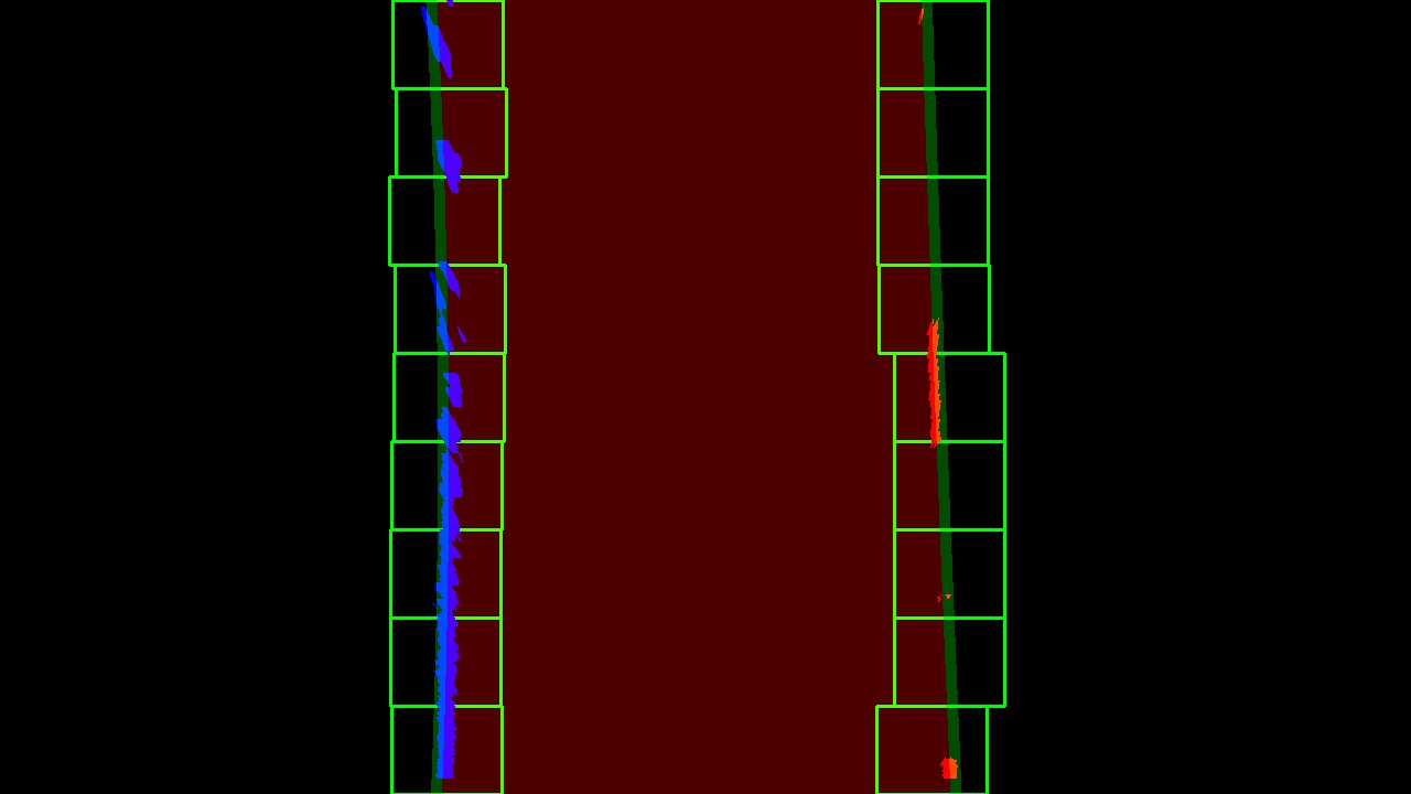
I used two methods to identify lane pixels. If there is no previous information, I use a window searching method similar to the one we learned in the lessons. If we have previous information, I search around the previous polynomial. I implemented a sanity checking method to make sure things didn't get too out of hand. Sample output here: 
This code is nearly identical to what we learned in class. If the lane object has a previous polynomial fit, and the recent frames have been identified successfully, then I search around the previous polynomial and fit a new polynomial the points that have been found.
I have added a sanity check to this (lines 73 to 76). See detailed description below in this document's line 120.
First part: Identify the likely positions of the lane lines in the image (lines 102-143): This method falls somehwere between the convolution and histogram search shown in the lectures. In the lesson, we separate the image into two and take the max on each side. I wanted to find all possible lane markers, including those from adjacent lanes. So, instead of taking the max from each half of the image I ran sliding windows across the image to find peaks in the histogram. I could have found sums in the windows which is the equivalent of convolution. It works out to the same. then, after I've found all potential lines, I take the nearest one on the left and the nearest one on the right for further analysis
Second part: using the starting points from the previous method, run windows vertically and find points. I more or less copied the function from our lessons. You can find it in line 146 of the Pipeline cell, which references the corresponding helper function.
Third part: fit a polynomial. Line 149. Again, very similar to what we learned in the lessons. References the relevant helper function.
Fourth part: Sanity check. I call a sanity check on each of the two lane lines (pipeline cell, lines 152 an 153), and then another sanity check on the full lane with the two lines (pipeline cell line 154). To implement this sanity check I created two helper functions.
- Line_is_ok() - you can find it in the Helper Function cell at line 263. This function checks that the X values from the recent fit are reasonable. Are they close to their previous values? If so (line 282), then I update the line's values with the latest. If not, and we've only missed a few frames, then I simply stick with the most recent values and updated an iterator (line 306-307). If however we've had poor line ids for more than a certain threshold (line 311), I reinitialize our line object and essentially force a window search the next time around.
- lane_is_ok() - you can find it in the Helper Function cell at line 316. I had high hopes for checking the polynomial coefficients, but in the end, I just do two basic checks. Firstly, that both lines passed the individual line sanity check in Line_is_ok(). Secondly, I make sure they don't cross. If there is a problem with the lane, then I don't output the overlay to the original image. For exapmle. if you check
of the challenge video, you'll see that I don't identify the right lane marker for the first few seconds, and as a result, I do not output the lane overlay.
In the Line_is_ok() sanity check function, line 299 of the helper function cell, you'll see that I calculate an average of the polynomial first from the past 3 valid readings (if we have 3 valid readings since the object has been initialized). This smooths out the fitting. You can see that when I calculate the lane overlay for the original image, lines 171 and 174 of the Pipeline cell, I used the Best_Fit which holds the average, and not the most recent fit.
5. Describe how (and identify where in your code) you calculated the radius of curvature of the lane and the position of the vehicle with respect to center.
I did this in lines 186 through 204 in the pipeline cell of the Jupyter notebook. I only implement this calcualtion if the sanity check has been successful. If either line or the whole lane seems unreasonable, I skip this step.
I hard coded ym_per_pix as 3/(405-288) based on the pixel length of a lane marker in the warped image. xm_per_pix is calculated as 3.7 meters divided by the width of the most recent fitting. (line 190 in the Jupyter notebook)
For the curvature calculation, I reference a helper function that is identical to the one we developed in the lessons. You can find the helper function in the Helper Cell line 201.
For the offset calculation, I do it inline. Essentially, I unwarp the polyfits for the right and left lane markers. I take their initial position closest to the vehicle. By calculating their midpoint, and assuming that 640 is the ideal midpoint, I can calculate the offset.
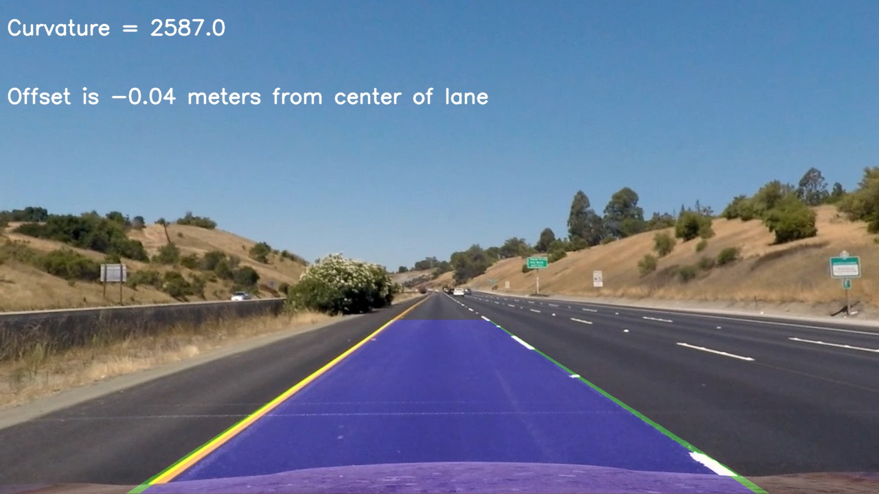
6. Provide an example image of your result plotted back down onto the road such that the lane area is identified clearly.
You can see the output in  First I created an overlay in warped space. I used polylines to draw green 2nd order polynomials for the two lane lines, and I used filllpoly to color the sapce between them in blue. (Pipeline cell, lines 167-178). I needed some help with syntax and found support in source j above.
In lines 180-183 I unwarped this overlay.
And in lines 208-212 I addweighted the overlay to the original image with additional text on curvature and offset.
1. Provide a link to your final video output. Your pipeline should perform reasonably well on the entire project video (wobbly lines are ok but no catastrophic failures that would cause the car to drive off the road!).
The project video can be found in and the challenge video can be found in
1. Briefly discuss any problems / issues you faced in your implementation of this project. Where will your pipeline likely fail? What could you do to make it more robust?
Some issues:
-
combination of color and gradient filters: I think I did a decent job. The project video and challenge video look good, but there are a few frames in the challenge video where the right lane marker isn't picked up. I think tweaking the color/gradient filters would help here.
-
efficiency: This algorithm is much slower than the first project. It defintiely does not run in real-time. WOuld be interested to know if there are tricks to make it better.
-
Sanity checker: I implemented some simple functionality to verify the sanity of individual lane lines and the lane as a whole. There are some edge cases that I know I've missed. I also think my threshold for forcing a restart of the window search isn't optimized. In short, there is a sanity checker, but with more time, I could make it better.
-
Additional lane lines: The gradient of R does a good job of picking up lines in adjacent lanes, and even the road edge in some cases. I dind't have the chance now, but I would like to trace those lines as well. It might even be possible to use the gradient as a separate image, so that it doesn't pollute the search for the main lane lines.
-
Harder challenge: I didn't do a great job with this one. I think my filters do a good job of picking out the lines, even in shadows, but the fitting isn't great. There are two changes I would implement. 1) I'd use a Hough Transform to dynamically identify lines for our bird's eye view transformation matrix. This would get the curved lane lines straight in the warped image. 2) I think we'd need a 3rd order polynomial fit at the least.

