Garabito/ScaraRobotControl

modelado y control de un robot scara

Presentation Project

Here is the study of the control of a 3-axis SCARA robot in this project. In a concern of simplification, we will only be interested in the robot's first two degrees of freedom. These degrees of mobility are associated with two pivot-type joints located in a horizontal plane. The joint coordinates of the robot are $\theta_1$ and $\theta_2$. These coordinates are subject to constraints (mechanical stops) The end effector is identified in space by its Cartesian coordinates. Restrictions on the joint coordinates induce a restricted domain reachable for the effector. In the Cartesian coordinate system, this domain is called the workspace or the operational space of the robot. The command of this robot is realized here by two DC motors, driven independently, coupled to reducers and amplifiers current. The main features of this robot are then given below:

• Two arms (considered as rods): $L_1 = 0.5m,L_2 = 0.4m,m1 = 5 kg$ and $m2 = 4 kg$
• Two GR80X80 motors, with an electromechanical time constant of 11.5 ms, rotational inertia J = 3200gcm²
• Two-stage ratio reduction $n_1 = n_2 = 100$
• Mechanical stops used throughout the project: $\theta_1$ between 0 and 270° and $\theta_2$ between -90° and 90°

Dynamic Control

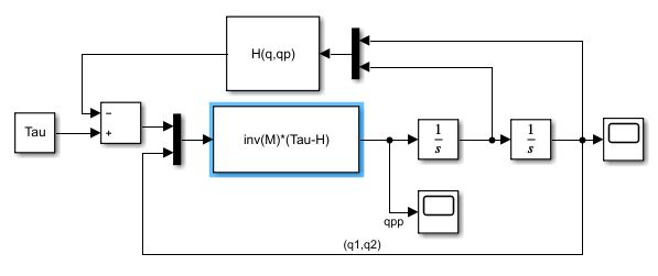
Here we compare several control laws using the dynamic model of our robot on Simulink. To do this, we use the following direct dynamic model. Of course, without correction, the joint variables tend to diverge since we only add in constant torque input. $$\ddot{q} = M(q)^{-1}(\Gamma-H(q,\dot{q}))$$

Dynamic Model

Proportional-Derivative (PD) Control

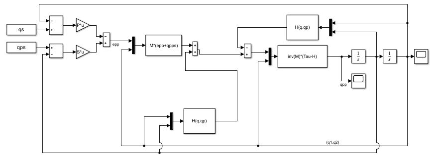
The proportional corrector makes it possible to stabilize the system, increase the speed, and reduce the error. A derivative corrector is added to this to reduce the oscillations. The main criterion of speed is limited by the electromechanical time constant of the robot motors of 11.5 ms. We give as input the position as well as the desired speeds, using:

$$ \Gamma(t)=K_P(q^s(t)-q(t))+K_D(\dot{q}^s(t)-\dot{q}(t)) $$

Proportional-Derivative (PD) Control

Linearized Control

We want to compare the Proportional/Derivative control to another nonlinear control law this time: a linearized control. This command consists in imposing a dynamic on the error e (error with respect to a trajectory). This dynamic is given by the equation:

$$ \ddot{e} = [M(q)]^{-1}(\Gamma - H(q,\dot{q}))-\ddot{q}_{ref} \hspace{5mm} and \hspace{5mm} \ddot{e} = S\dot{e}-Pe $$

Inverting this equation to find the control input:

$$ \Gamma = [M(q)](\ddot{e} + \ddot{q}_{ref}) + H(q,\dot{q}) $$ We can thus adjust $\ddot{e}$ in order to ensure stability and trajectory tracking performance by playing on the S and P gains. To simplify the representation, it is useful to take an acceleration setpoint from the variables zero joints.

Linearized Control

Mathematics Model

Geometric and kinematic models

The direct geometric model of the robot is expressed through the Denavit-Hartenberg parameter method.

$$ \left{ \begin{array}{ll} x = L_{2}cos(\theta_{12}) + L_{1}cos(\theta_{1}) \\ y = L_{2}sin(\theta_{12}) + L_{1}sin(\theta_{1}) \end{array} \right. $$

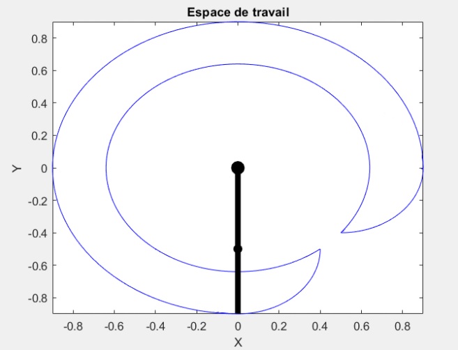
Operational Space of the end effector

Inverse geometric model

We express the inverse geometric model to obtain the expression of the joint variables $(\theta_1, \theta_2)$ as a function of the operational variables (x, y) Thanks to the inverse geometric model, we find the values of the corresponding joint variables to achieve any trajectory (see for example the following linear trajectory).

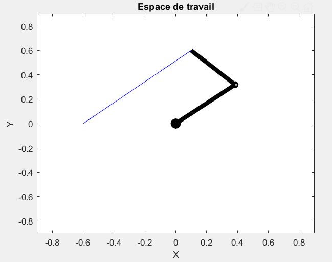
Linear trajectory

Direct Kinematic Model

The direct kinematic model expresses the velocities of the operational variables as a function of the velocities of the joint variables. To obtain this model, we calculate the Jacobian matrix. It is given by the successive partial derivatives with respect to the joint variables.

$$ \left{ \begin{array}{ll} x = L_{2}cos(\theta_1+\theta_2) + L_{1}cos(\theta_{1}) \\ y = L_{2}sin(\theta_1+\theta_2) + L_{1}sin(\theta_{1}) \end{array} \right. $$ $$ \begin{equation} J(q) = \begin{pmatrix} -L_1sin(\theta_1)-L_2sin(\theta_1+\theta_2) & -L_2sin(\theta_1+\theta_2) \ L_1cos(\theta_1) + L_2cos(\theta_1+\theta_2) &L_2cos(\theta_1+\theta_2) \end{pmatrix} \end{equation} $$

Inverse Kinematic Model

The inverse kinematic model expresses the joint velocities as a function of those of the operational coordinates. It is found by calculating the inverse of the Jacobian matrix (find the details in the handout).

For a square Jacobian matrix, as found previously, it is desirable to study its rank and determinant to highlight the possible points of singularity.

$$ det(J) = L_1L_2 sin(\theta_2) $$ $$ det(J) = 0 \xrightarrow[]{} L_1L_2sin(\theta_2)=0 \xrightarrow[]{} \theta_2 = 0[k\pi], k \in \mathbb{Z} $$

Therefore, we have singularities with the values of $\theta_2 = 0$ and $\pi$ and their multiples. This means that if during a trajectory $\theta_2$ approaches these values, the joint speed will tend towards infinity (which should be avoided). Using those geometric and kinematic models, we can easily perform trajectory tracking, avoiding singular points.

Dynamic Model

We use the formalism of Lagrange, which is based on the calculation of the energy, to determine this model.

Operational Space of the end effector

$$ \Gamma= M(q)\ddot{q}+H(q,\dot{q}) $$

$$ M=\begin{bmatrix} \frac{J_{m1}}{n_1}+\frac{5}{12}m_1l_1^2+m_2(l_1^2+\frac{5}{12}l_2^2+l_1l_2 cos(\theta_2)) & m_2(l_1^2+\frac{5}{12}l_2^2+l_1l_2cos(\theta_2)) \\ m_2(l_1^2+\frac{5}{12}l_2^2+l_1l_2cos(\theta_2)) & \frac{J_{m2}}{n_2}+m_2(l_1^2+\frac{5}{12}l_2^2+l_1l_2cos(\theta_2)) \end{bmatrix} $$

$$ \hspace{3cm}H=\begin{bmatrix} -m_2 \hspace{1mm} l_1l_2\dot{\theta_2}sin(\theta_2)\hspace{1mm} (\dot{\theta_1}+\dot{\theta_2}) \\ - \frac{m_2}{2}l_1l_2sin(\theta_2)\hspace{1mm} (\dot{\theta_2}^2-\dot{\theta_1}^2) \end{bmatrix} $$

Instructions for use :

• Launch the visualization_trame.m script for the first time to create the variables in the workspace (You might have errors at the end of the program because the simulation files are not yet created)
• Make run section 12
• Open the Simulink model and launch the simulation and visualize the results 12 in the scope
• Make run section 14
• Then run section 15, open the Simulink qu15 model and run the simulation
• Run section 15b to visualize the trajectory in a circle
• Change the value of mc and run section 16
• Return to the main Simulink and launch the simulation to perform the calculation with mc different from 0
• Run section 16b to visualize trajectories with the addition of mass
• Run section 17 to visualize the effect of disturbances