Gradient Descent Algorithms

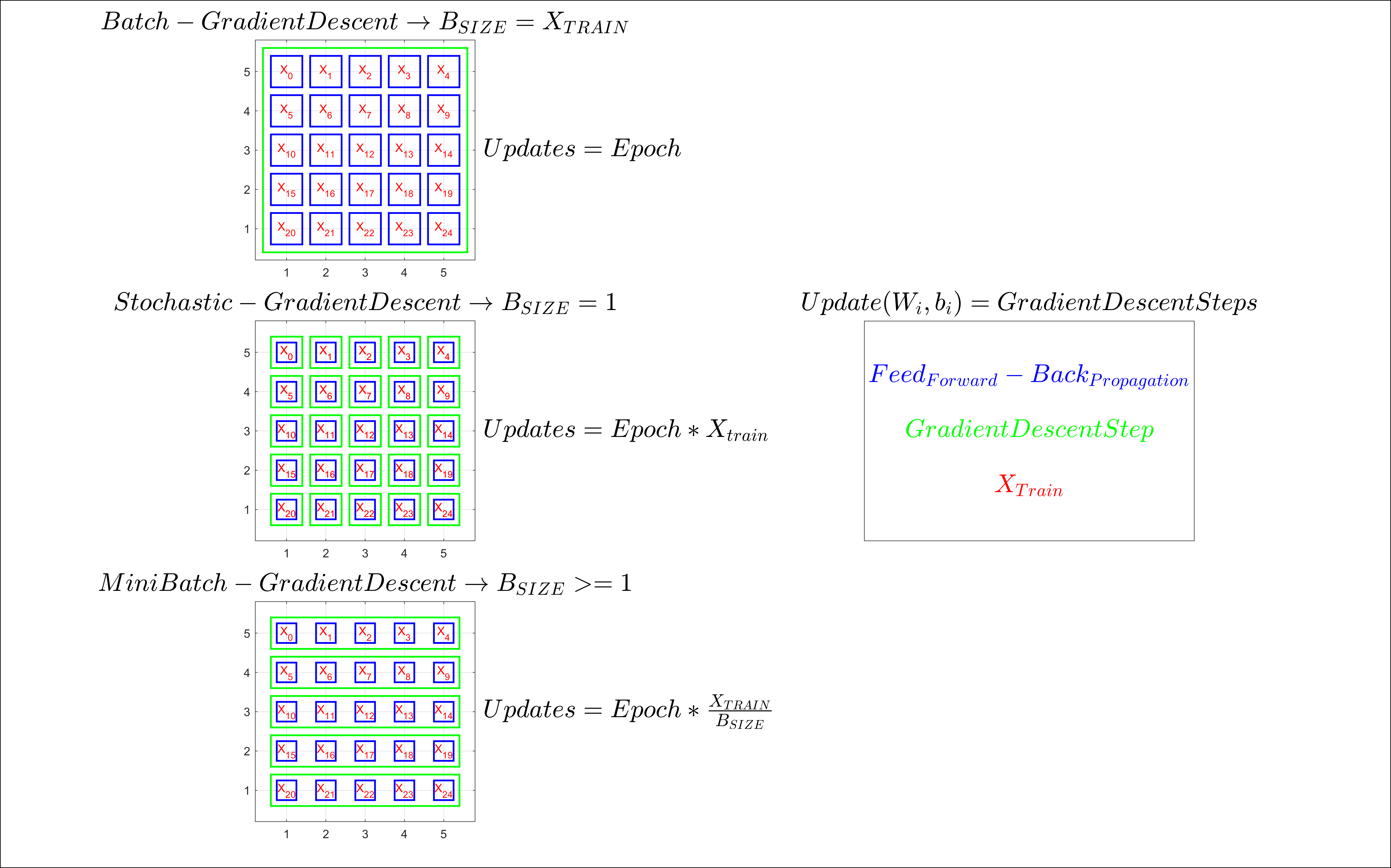
Batch Gradient Descent.
Stochastic Gradient Descent.
Mini-Bach Gradient Descent.

# MINI BACH GRADIENT DESCENT
for epoch in n_epochs:
    for batch in n_batches:
        for all instances in the batch  
            #compute the derivative of the cost function
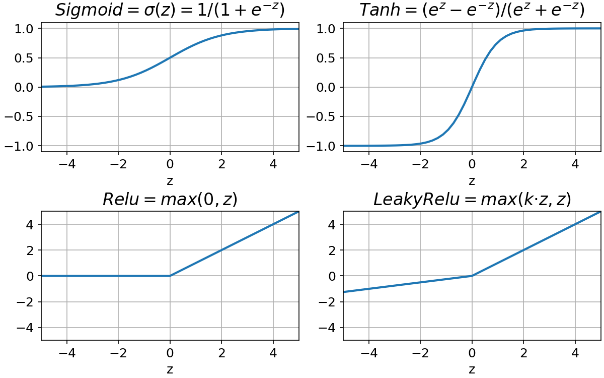
        #update the weights and biases

Derivatives on Computational Graphs

$\frac{\partial{Z}}{\partial{X}} \rightarrow$ Sum over all possible paths between node $X$ and node $Z$, multiplying the derivatives on each edge of the path together.

Net feed forward Matrix Dimensions

Activation functions

Tanh improves sigmoid function because with sigmoid all the weights of the same neuron must increase or decrease together as the activations will always be positive and the sign will depend on the error associated with the neuron. With Tanh the activations in the hidden layers would be equally balanced between positive and negative values.

$$ \frac{\partial C}{\partial W^l} = \delta^l [a^{l-1}]^T $$

Feed forward activations: Single Neuron

$$a^{l}_j = \sigma \bigg( \sum_k w^l _{jk} a^{l-1}_k + b^l_j \bigg)$$

$w_{jk}$ denote the weight for the connection from the $k \textrm{ } neuron$ in the $(l−1)$ layer to the $j \textrm{ } neuron$ in the layer $l$.

In vectorized form:

$$a^l = \sigma \bigg( W^la^{l-1}+b^l \bigg)$$

Gradient vector of the cost function

$$TrainingInputs=x_1, x_2, \ldots,x_n$$

$$MiniBatches=[X_1, X_2, \ldots,X_m],[X_1, X_2, \ldots,X_m]...$$

$$\nabla C = \frac{1}{n}\sum_{x=1}^n\nabla C_x \approx \frac{1}{m} \sum_{j=1}^m \nabla C_{X_{j}} $$

$$\nabla C \approx \frac{1}{m} \sum_{j=1}^m \nabla C_{X_{j}}$$

Update W,b using Gradient Descent

$$w_k \rightarrow w_k-\eta \frac{\partial C}{\partial w_k}$$

$$b_l \rightarrow b_l-\eta \frac{\partial C}{\partial b_l}$$

Update W,b using Stochastic Gradient Descent with Mini-Batches

$$w_k \rightarrow w_k-\frac{\eta}{m}\sum_j \frac{\partial C_{X_j}}{\partial w_k}$$

$$b_l \rightarrow b_l-\frac{\eta}{m}\sum_j \frac{\partial C_{X_j}}{\partial b_l}$$

Backpropagation

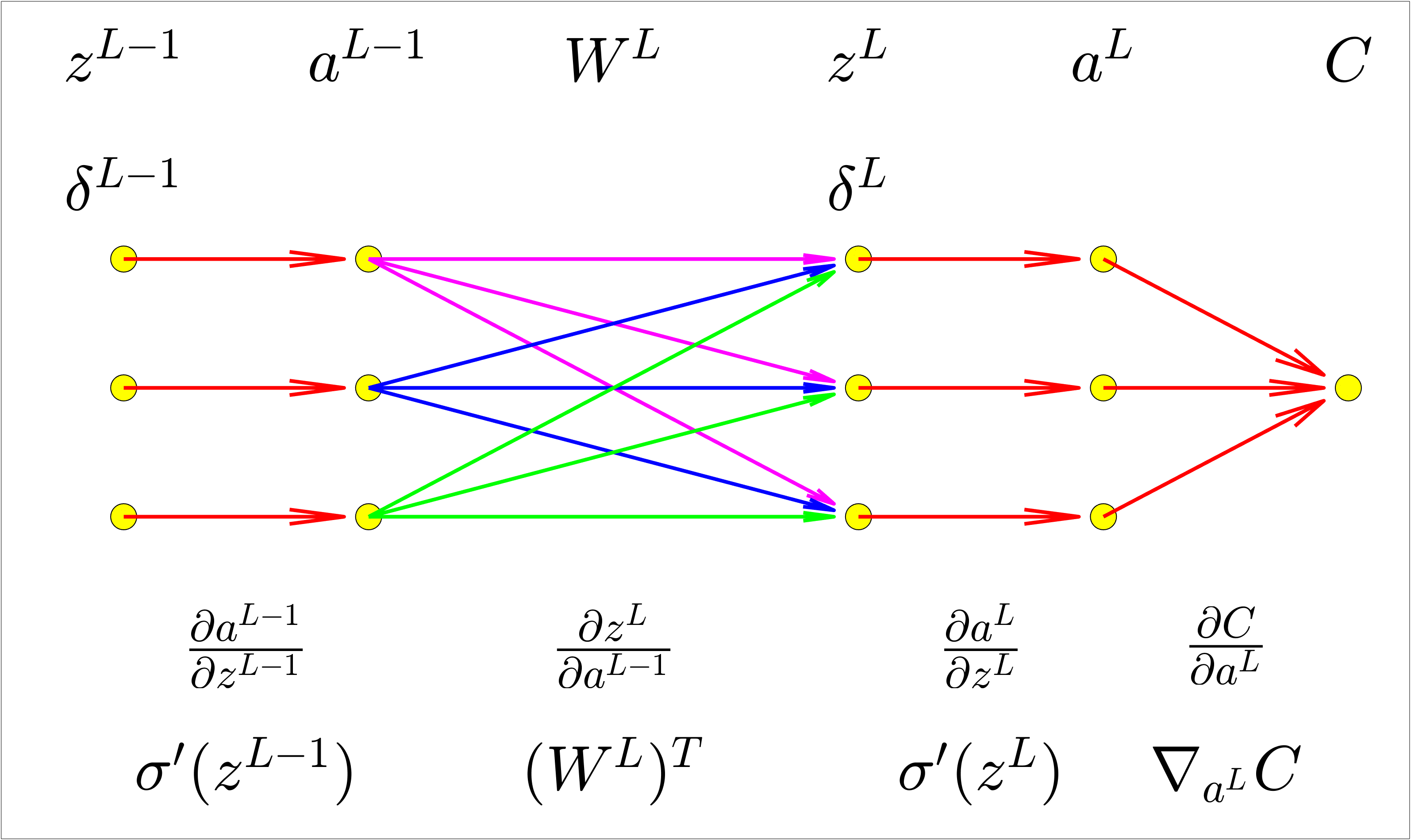
Backpropagation compute:

The partial derivatives $\partial C_x/ \partial W^l$ and $\partial C_x/ \partial b^l$ for a single training input. We then recover $\partial C/ \partial W^l$ and $\partial C/ \partial b^l$ averaging training examples on the mini bach.
$Error$ $\delta^l$ and then will relate $\delta^l$ to $\partial C/ \partial W^l$ and $\partial C/ \partial b^l$.
Weight and Biases will learn slowly if:
- The input neuron is low-activation $\rightarrow a^{l-1}_k$.
- The output neuron has saturated $\rightarrow \sigma'(z^l)$
Backpropagation Equations:

$$ \begin{align} & \delta^L = \frac{\partial C}{\partial z^L} \\ & \\ & \delta^L = \nabla_{a^L} C \odot \sigma'(z^L) \\ & \\ & \delta^l = ([W^{l+1}]^T \delta^{l+1}) \odot \sigma'(z^l) \\ & \\ & \frac{\partial C}{\partial W^l} = \delta^l [a^{l-1}]^T \\ & \\ & \frac{\partial C}{\partial b^l} =\delta^l \\ \end{align} $$

Gradient Descent Combined with Backpropagation

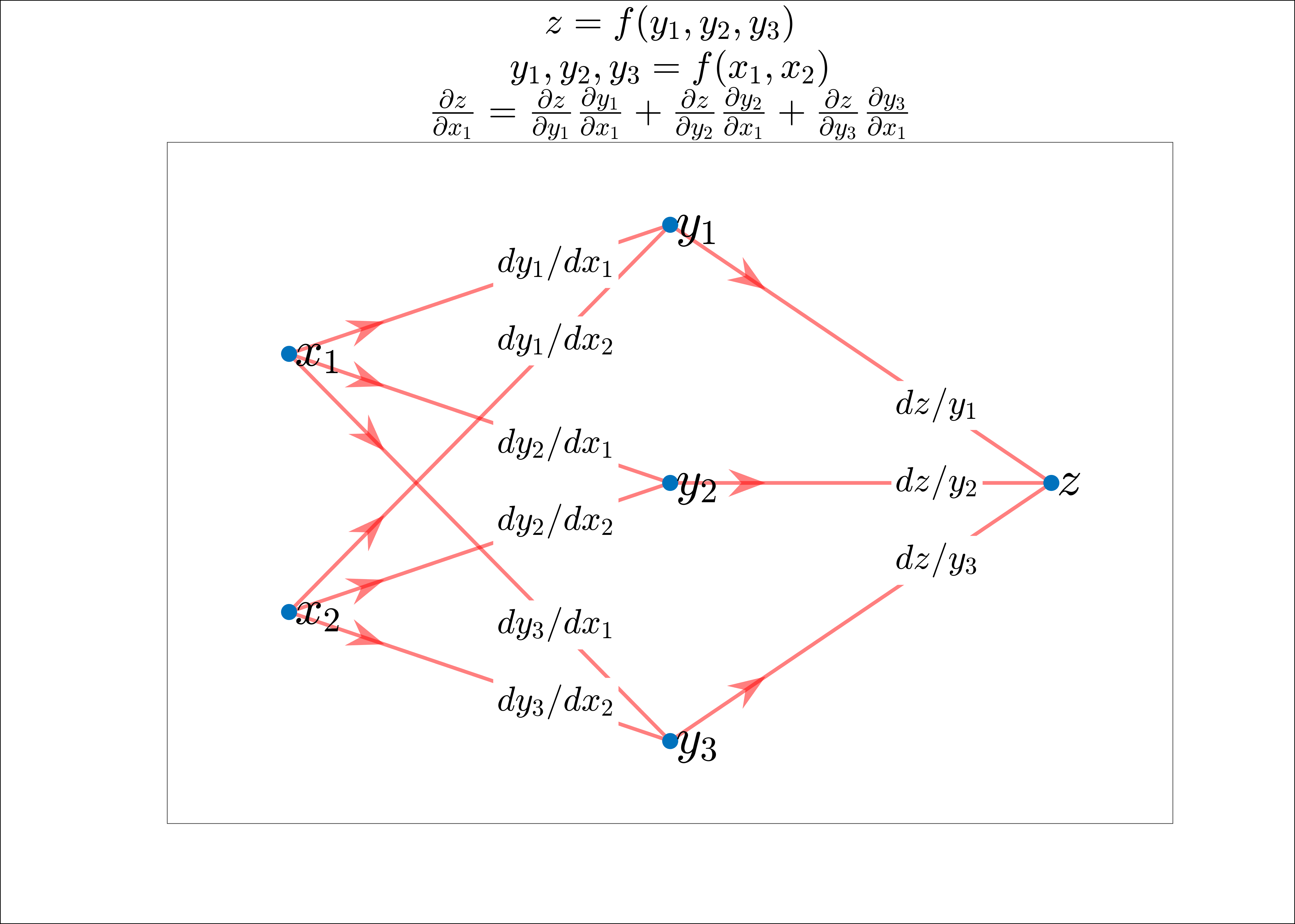
$$ \begin{align} & W^l \rightarrow W^l -\frac{\eta}{m} \sum^m_x \delta^l_x [a^{l-1}_x]^T \\ & \\ & b^l \rightarrow b^l -\frac{\eta}{m} \sum^m_x \delta^l_x \\ \end{align} $$

Chain rule applied in Backpropagation

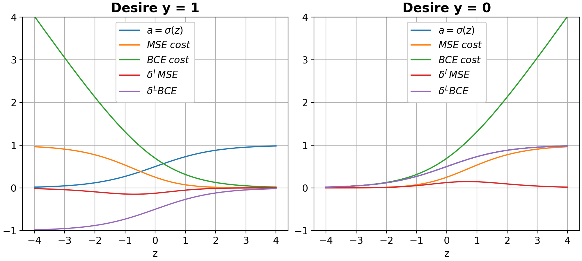
Binary cross entropy cost function: Avoid slow training

$$ a=a^L =\sigma(z^L) $$

Quadratic Cost $MSE$: Often used in regression problems where the goal is to predict continuous values.
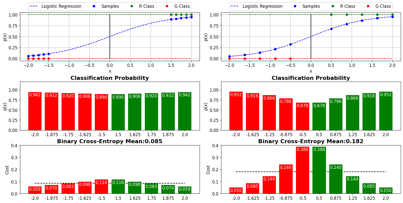
Binary Cross-Entropy $BCE$: Often used in classification problems where the goal is to predict discrete class labels

$$ \begin{align} & C_{MSE} = \frac{1}{2n} \sum_x ||y-a^L||^2 \\ & \\ & C_{BCE} = -\frac{1}{n} \sum_{x}\sum y \ln a^L+(1-y) \ln(1-a^L) \\ \end{align} $$

Derivatives :

$$\frac{\partial C_{MSE}}{\partial W^L} = \underbrace{ (a^L-y) \sigma'(z^L) }_{\delta^L}[a^{L-1}]^T$$

$$\frac{\partial C_{BCE}}{\partial W^L} = \underbrace{ (a^L-y) }_{\delta^L}[a^{L-1}]^T$$

When the weights are updated using the CE cost function it does not matter if the neurons are saturated $\sigma'(z^L) \approx 0$ since the derivative term is avoided. The rate at which the weight learns is controlled by the error $(a^L-y)$. The larger the error, the faster the neuron will learn. The cross-entropy function is demonstrated from the following equations. The quadratic cost learning is slower when the neuron is wrong, while with the cross-entropy learning is faster when the neuron is wrong

$$ \begin{align} & \sigma(z) = 1/(1+e^{-z}) \\ & \\ & \sigma'(z) = \sigma(z)(1-\sigma(z)) \\ \end{align} $$

Logistic Regression and Binary Cross Entropy Cost

Entropy: $H(p)$
Cross Entropy: $H(p,q)$

$$ \begin{align} & H(p) = -\sum_x p(x) \log(p(x)) \\ & \\ & H(p,q) = -\sum_x p(x) \log(q(x)) \\ \end{align} $$

Softmax

The activation function of the last layer can be thought of as a probability distribution. It can be useful with classification problems involving disjoint classes.

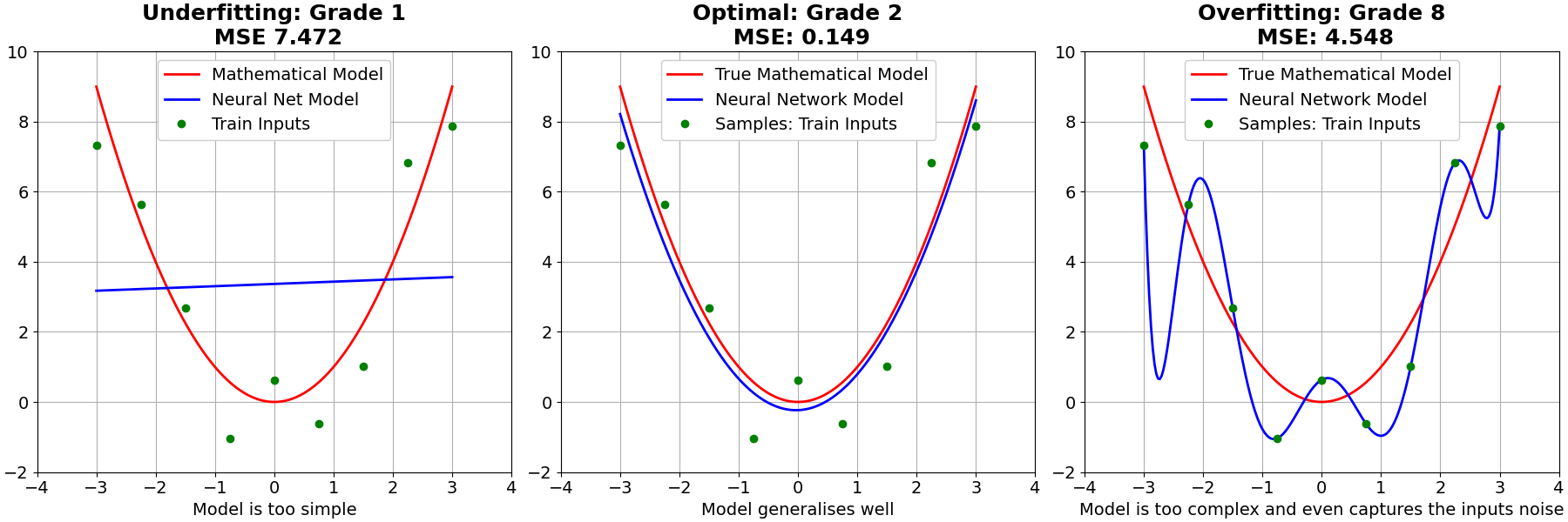
$$ \begin{align} & a^L_j = \frac{e^{z^L_j}}{\sum e^{z^L_j}} \\ & \\ & \sum a^L_j = 1 \\ \end{align} $$

Regularization: Decrease overfitting and Generalise better

The effectis to make it so the network prefers to learn small weights. Large weights will only be allowed if they considerably improve the first part of the cost function. Regularization can be viewed as a way of compromising between finding small weights and minimizing the original cost function. The relative importance of the two elements of the compromise depends on the value of $\lambda$. When $\lambda$ is small we prefer to minimize the original cost function, but when $\lambda$ is large we prefer small weights. Instead of simply aiming to minimize loss (empirical risk minimization) we'll now minimize loss+complexity, which is called structural risk minimization:

$$\text{minimize( Loss(Data|Model) )}$$ $$\text{minimize( Loss(Data|Model) + complexity(Model) )}$$

$L1:$

$$ \begin{aligned} & C = C_0 + \underbrace{ \frac{\lambda}{n} \sum_w |w| }_{L1} \\ \end{aligned} $$

$L2:$

$$ \begin{align} & C = C_0 + \underbrace{ \frac{\lambda}{2n}\sum_w w^2}_{L2} \\ \end{align} $$

Regularized networks are constrained to build relatively simple models based on patterns seen often in the training data, and are resistant to learning peculiarities of the noise in the training data.Thus, regularised neural networks tend to generalise better than non-regularised ones.

Regularization and gradient descent

The dynamics of gradient descent learning in multilayer nets has a ``self-regularization effect´´.

$L1:$

$$ \begin{align} & C = C_0 + \frac{\lambda}{n}\sum_w |w| \\ & \\ & \frac{\partial C}{\partial w} = \frac{\partial C_0}{\partial w} + \frac{\lambda}{n} sgn(w) \\ & \\ & w \rightarrow w - \eta \frac{\lambda}{n} sgn(w) - \frac{\eta}{m}\sum_j \frac{\partial C_{X_j}}{\partial w} \\ \end{align} $$

$L2:$

$$ \begin{align} & C = C_0 + \frac{\lambda}{2n}\sum w^2 \\ & \\ & \frac{\partial C}{\partial w} = \frac{\partial C_0}{\partial w} + \frac{\lambda}{n} w \\ & \\ & w \rightarrow w-\eta \frac{\partial C_0}{\partial w}-\eta\frac{ \lambda}{n} w \\ & \\ & w \rightarrow w-\eta \frac{\lambda}{n}w -\frac{\eta}{m} \sum_j \frac{\partial C_{X_j}}{\partial w} \\ & \\ &w \rightarrow \left(1-\eta \frac{\lambda}{n}\right)w -\frac{\eta}{m} \sum_j \frac{\partial C_{X_j}}{\partial w} \\ \end{align} $$

When a particular weight has a large magnitude $|w|$, $L2$ regularization shrinks the weight much more than $L1$ regularization does. When $|w|$ is small, L1 regularization shrinks the weight much more than L2 regularization.

Dropout

The dropout procedure is like averaging the effects of a very large number of different networks. The different networks will overfit in different ways, and so, hopefully, the net effect of dropout will be to reduce overfitting.

If we think of our network as a model which is making predictions, then we can think of dropout as a way of making sure that the model is robust to the loss of any individual piece of evidence. In this, it's somewhat similar to L1 and L2 regularization, which tend to reduce weights, and thus make the network more robust to losing any individual connection in the network

Weight Initialization

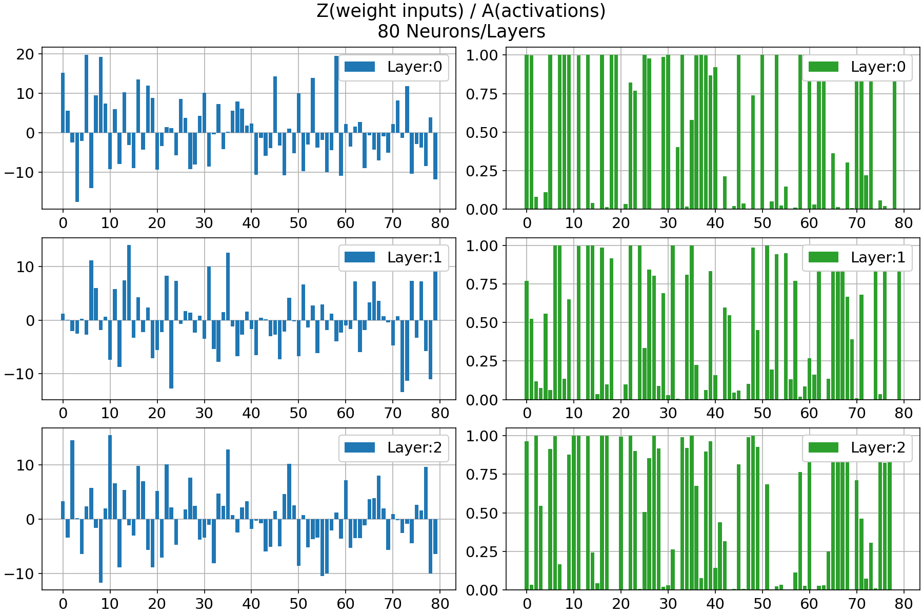
When the weights have a large magnitude, the sigmoid and tanh activation functions take on values very close to saturation. When the activations become saturated, the gradients move close to zero during backpropagation.

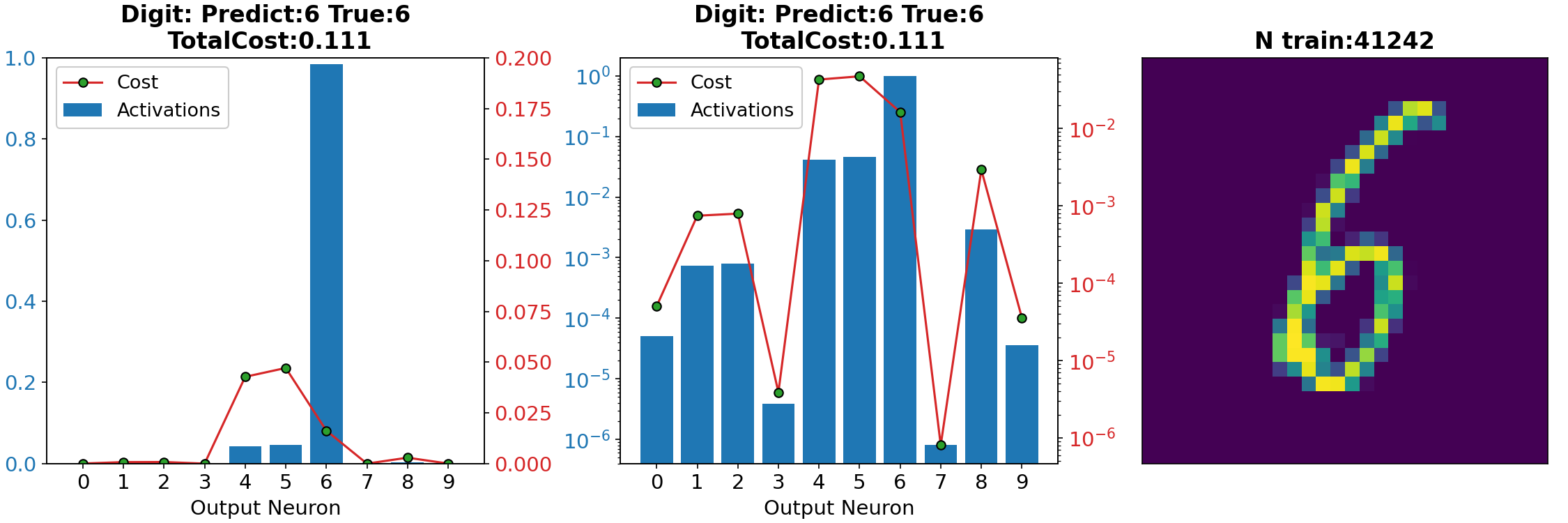
The problem of saturation of the output neurons causes a learning slowdown using the MSE cost function. This problem is solved using the BCE cost function.
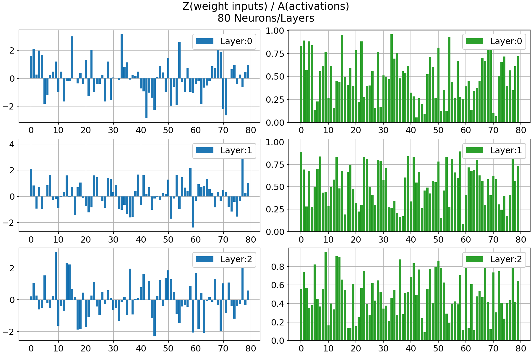
For the saturation of the hidden neurons this problem is solved with a correct weight initialization.

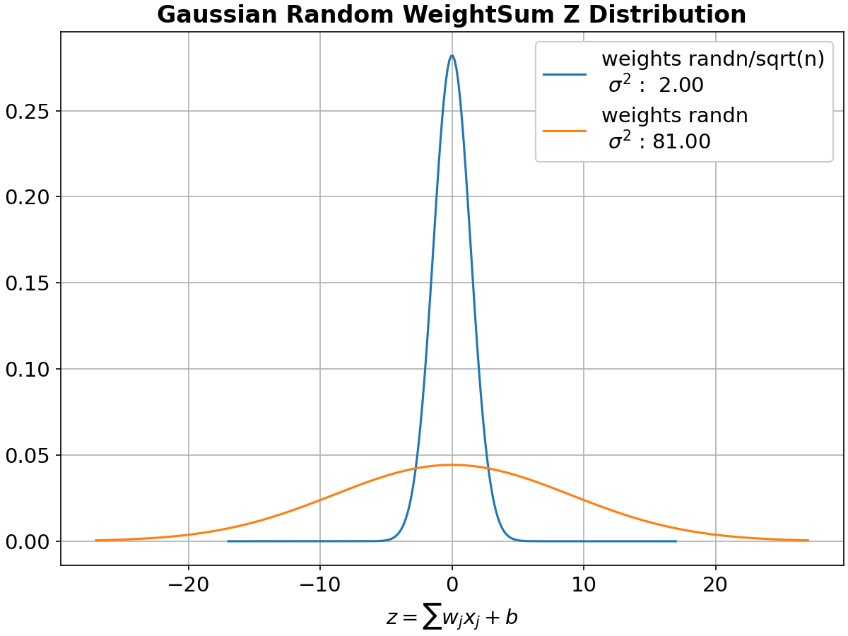
The idea is to initialize $Var(W)$ in a way that $Var(Z)$ remains roughly constant. This is where the $\frac{1}{\sqrt n}$ scaling comes in. By dividing the weights by $\sqrt n$, the variance of the weights is effectively scaled by $\frac{1}{n}$, ensuring that the variance of the output remains approximately 1 Sacaling the standard normal distribution by a constant $n$ effectively multiply the variance by $n^2$.

Standard Normal Distribution: The weights for each connection between input neurons and hidden neurons are drawn independently from a standard normal distribution $N(0,1)$ The mean of this distribution is 0, and the variance is 1.
Variance in Hidden Neurons: The variance in the hidden neurons is influenced by the weights connecting the input neurons to the hidden neurons. Since each weight is drawn independently from a standard normal distribution, the overall variance in the hidden neurons would be proportional to the number of input neurons.
Effect on Learning: While random initialization is crucial for breaking symmetry and promoting effective learning, initializing weights without scaling can lead to challenges such as vanishing or exploding gradients, especially in deep networks.

# randn
weights = [np.random.randn(r,c) for r,c in zip(rows,cols)]

# normalized
weights = [np.random.randn(r,c)/np.sqrt(c) for r,c in zip(rows,cols)]

Randn

Normalized

Choose a neural network's hyper-parameters

Reduce the number of classes and the test data
Decreasing training cost $\eta$: 0.1, 1.0, 2.5, 5
Validation accuracy: $\lambda$, $m$, $Nº$ $HiddenNeurons$
Early stopping to determine the number of training epochs: (Compute the classification accuracy on the validation data at the end of each epoch). Terminate training if the best classification accuracy doesn't improve for quite some nº of epochs

Recognize handwritten digits from MNIST dataset

Parts of the data set

# training_data = [(x1,y1),(x2,y2)...(xn,yn)]
# len = 50000
# xi  = array(784,1)
# yi  = array(10,1)

# test_data = [(x1,y1),(x2,y2)...(xn,yn)]
# len = 10000 
# xi  = array(784,1)
# yi  = number 0,1,2...9

# validation_data = [(x1,y1),(x2,y2)...(xn,yn)]
# len = 10000 
# xi  = array(784,1)
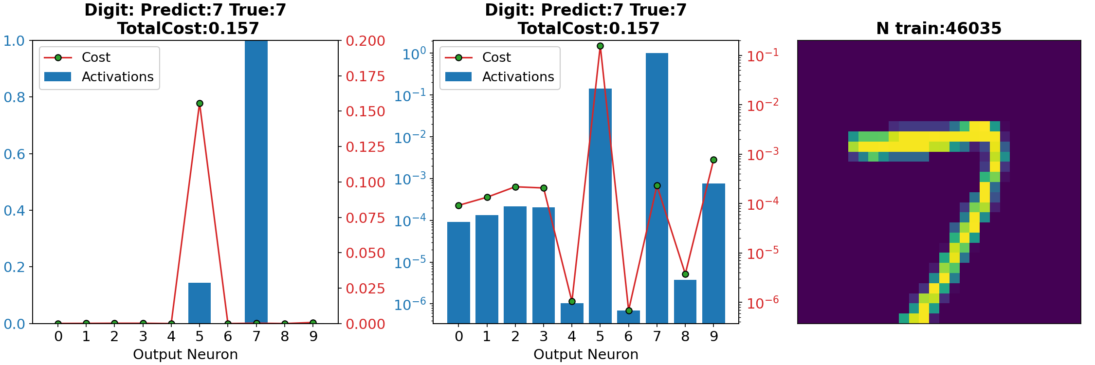
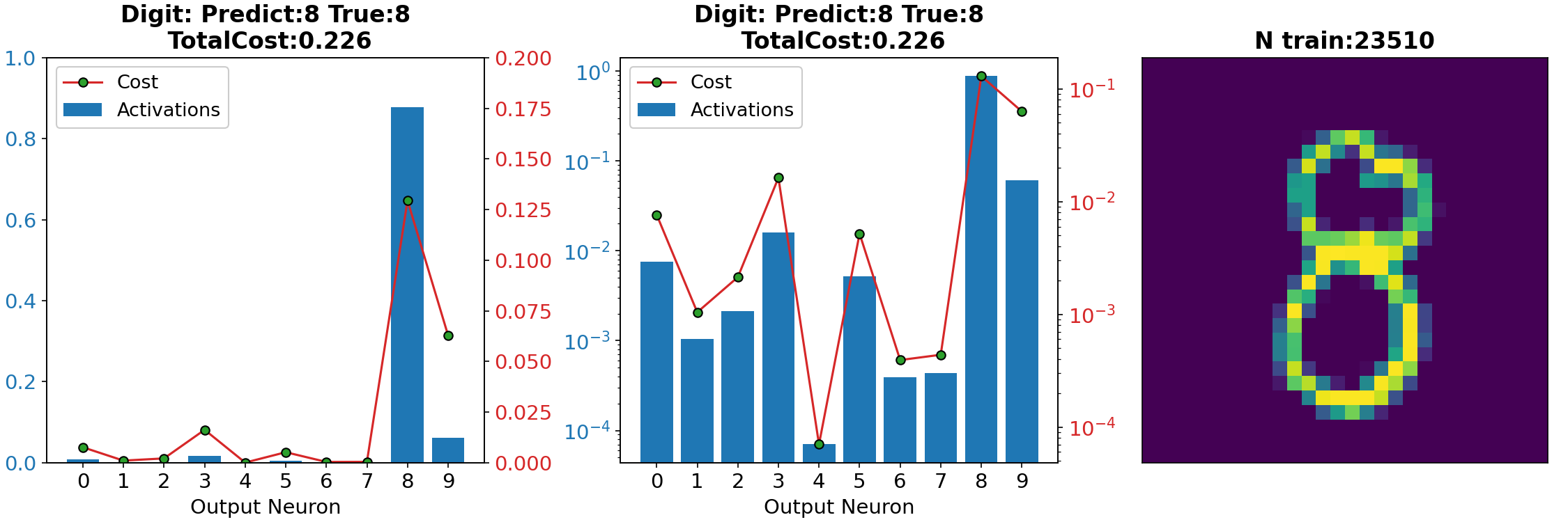
# yi  = number 0,1,2...9

Net output

n    = 100
x, y = training_data[n]
a    = net.feedforward(x)

# a: Net output
# array([[2.26639888e-03],
#        [3.91142856e-04],
#        [4.30652386e-05],
#        [2.98756664e-06],
#        [3.88572904e-04],
#        [9.06726417e-01], Digit 5
#        [1.95308412e-02],
#        [6.02094721e-06],
#        [8.41020120e-02],
#        [3.07447887e-02]])

# y: Desire output
# array([[0.],
#        [0.],
#        [0.],
#        [0.],
#        [0.],
#        [1.], Digit 5
#        [0.],
#        [0.],
#        [0.],
#        [0.]])

Examples with cost

2D point classification in circular and spiral geometries

Spirals

Circles

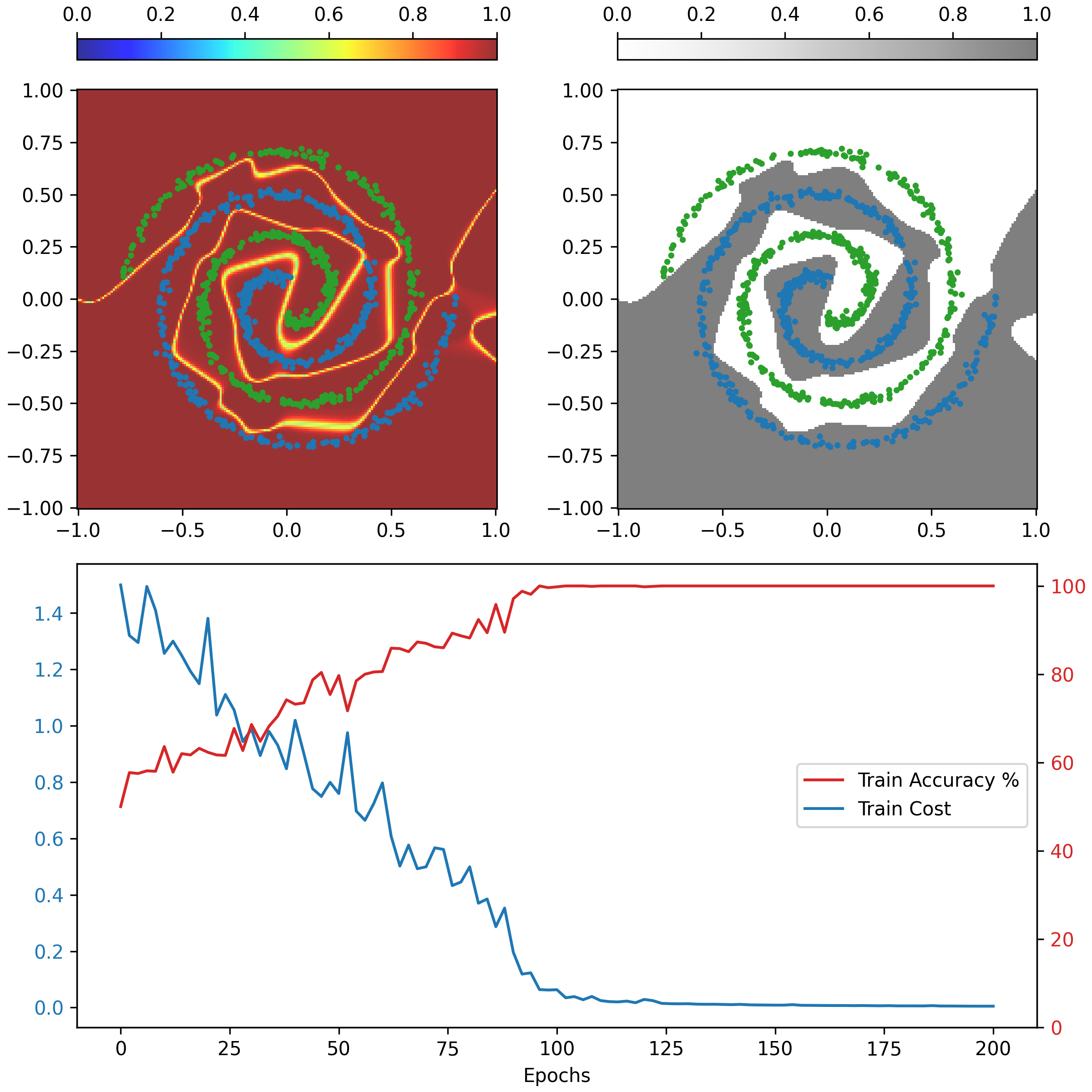
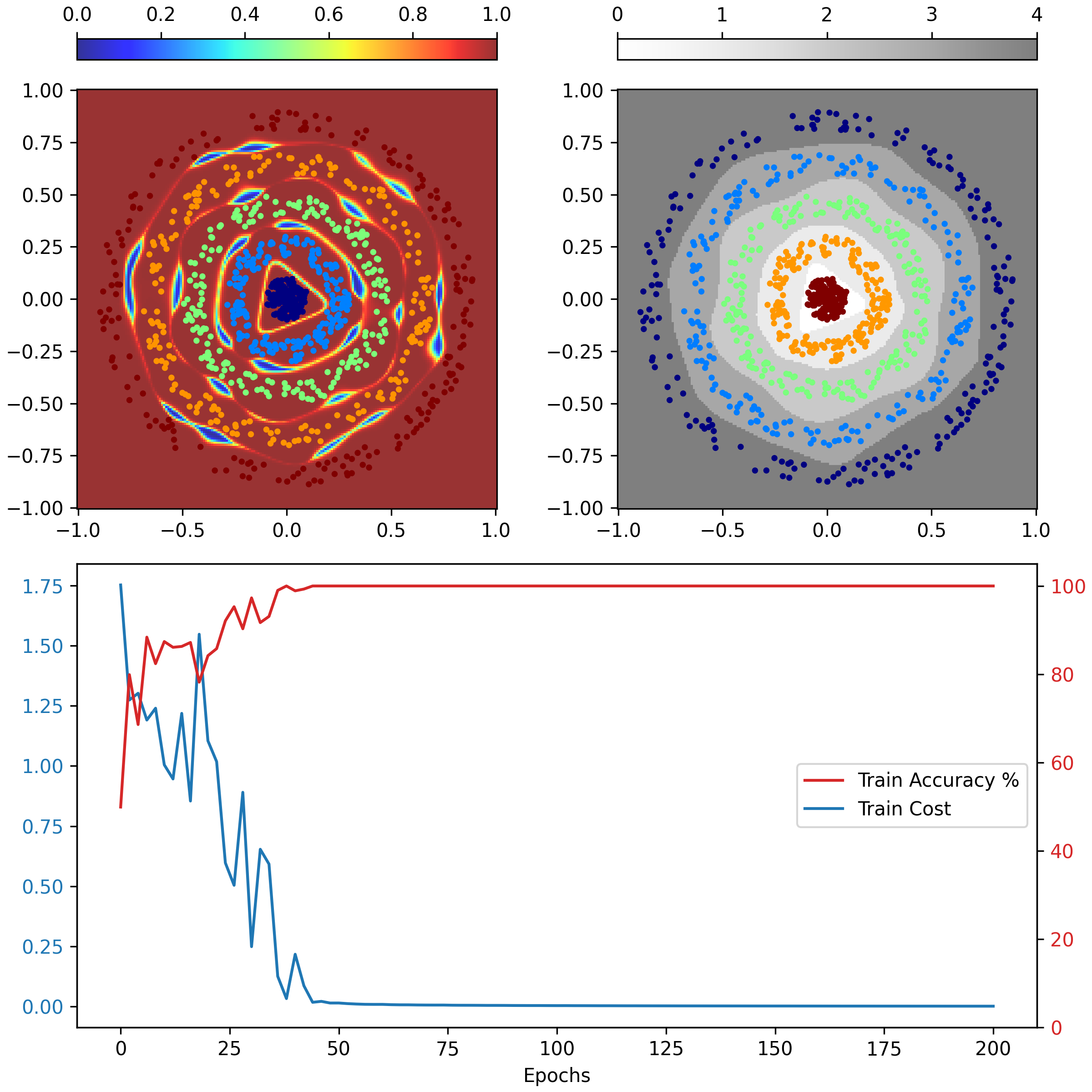
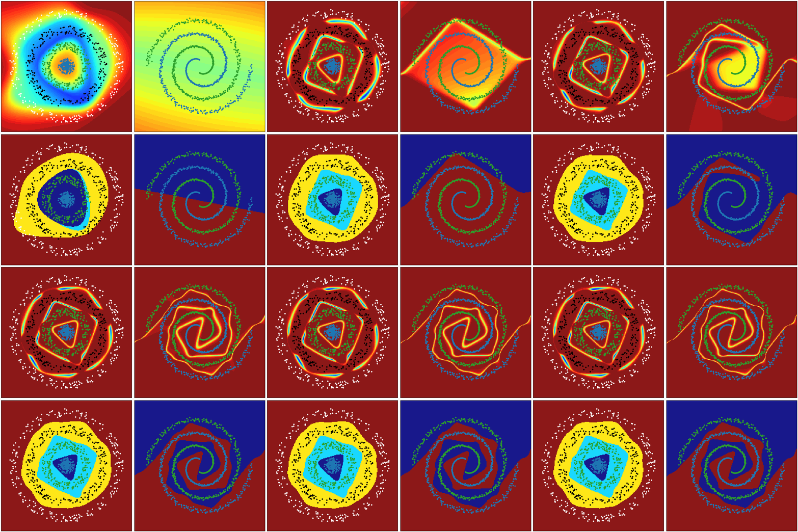
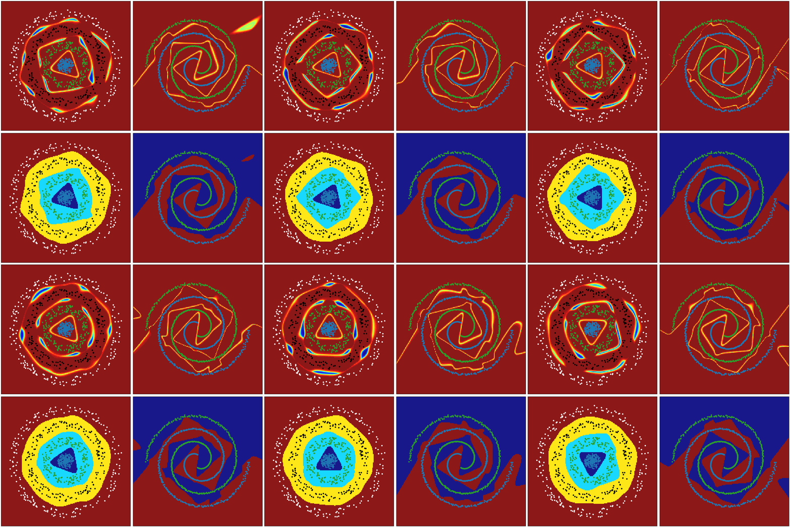
Animations

These animations show the ability of a Neural Network to transform the space in a non-linear way to create regions that allow to delimit and classify the input data. The colour gradient represents the normalised output of the network (first row) and the discrete colours represent the different classification regions (second row).

The first animation represents the evaluation of the network during the training process. The second one represents the evaluation after being trained, keeping the same architecture, hyperparameters, training data but different initialisations of weights.