This is popular task from Comma AI. Your goal is to predict the speed of a car from a video. More about the task https://github.com/commaai/speedchallenge.
We have 17 min training video, with 20 frames per second. It's 20400 frames, where we have speed on each frame. From the initial description, we can start with some basics on it a) Features taken from Images b) Features elapsed over time. We will include all work we had, and other possible thoughts.
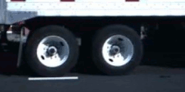
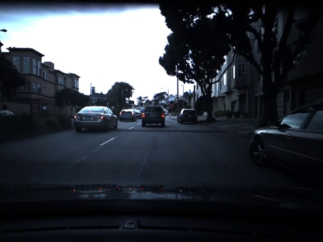
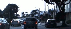
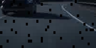
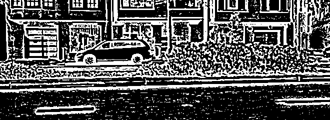
Start with checking training video, we will see highway varience 70% of the video, and street about 30 %. We do have some noises, like low distance between cars, and few turns with very smoothed rotation. Some examples of the frames, you can see below. Nothing special at all.
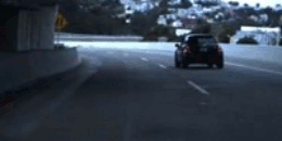
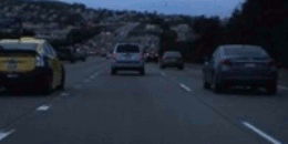
1.1.1. Examples of Working Areas in the train set.
However, we have existing video for testing. Test video have 9 min video with the same framerate, and will be used for the next model evaluation. As you will see, it's not just usual task, where you need to keep in mind a regularization objective. But think about alternatives for the feature extraction.
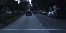
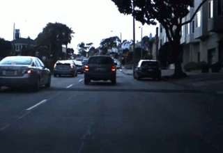
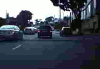
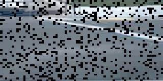
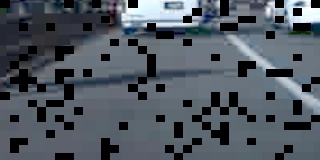
So lets describe test set, and what we have. Only 30% of varience from the highway. We have a lot of noises, which completely new comparing to the training set. Few of them are - Sharp turns - Car stop - Road steep descent and ascent.
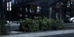
1.1.2. Examples of Working Areas in the test set. LTR Car turning Ex.1 - Car stop - Car turning Ex.2
We will start with check training data and it's changes over time. Most useful information, it's changes speed over time. You can see, where speed changes very swift, and we can use it for tracking anomaly detection for the next validation phase (when ever your predictions meet near to unexpected result).
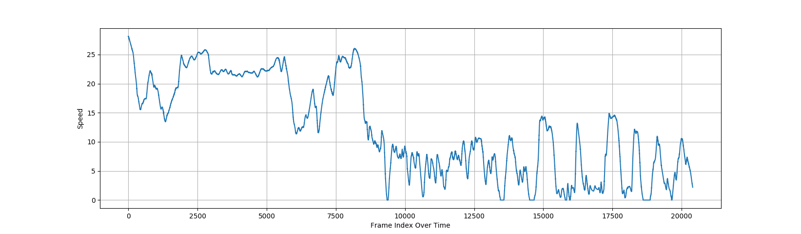
1.1.3. Speed value at Frame index from initial training Video.
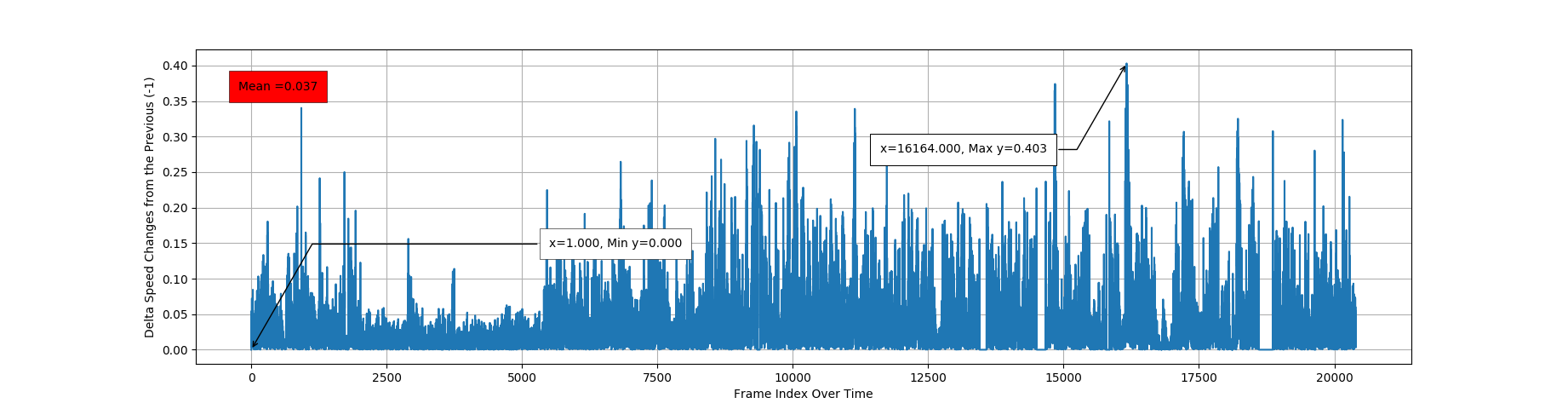
1.1.4. Delta Speed changes over Previous frame.
Above Image explains how Speed may change from the previous. Even one Video is not enough to relay on this value, we can assume this parameter is good for validation and checking anomalies in a prediction. One more sample, of avarage rate of changing Speed, over previous 20 frames (1 second in time).
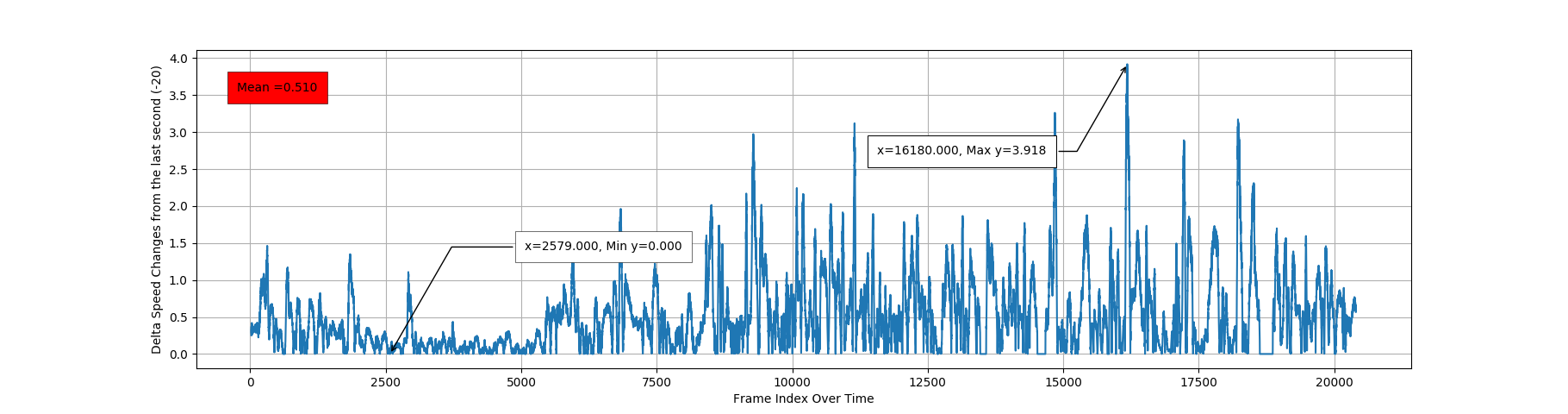
1.1.5. Delta Speed changes over Previous 20 frames.
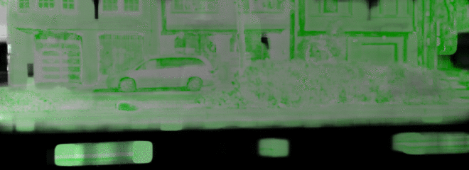
From each frame, we can decide working area, which includes most of the features, depending on our task. And reduce number of the Inputs. Even we did some feature area investigation, it's easy to manually retrive most useful part.
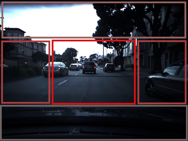
2.1.1. Source Image and Source Image Areas. Red Box represents Working Area, for the next steps.
But we have another interesting question here. As you can see, we have Working Area, which consist from some Sub Areas, Close and Far. First one, has more features about road changes (has more changes over time, due of camera angle). And Second one with more noise like side objects, other cars and less road changes.
2.1.2. Frame changes updates in different way, based on Angle of a Camera.
At this point, we have few variants, for next preprocessing steps. We will use this options in the next phases. - Using Far Sub Area. - Using Close Sub Area, and so on.
Note. It's very important to reduce number of Inputs, especialy in such cases, where we working with Video, and features elapsed over time. One wrong step will cause your model to have the Curse of Dimensionality. That is why we suppose to avoid last variant with using complete Working Area.
Below animation, how we can estimate it, with changes over time. Note, this sample only for visualizing and deciding about next steps. because correct Area we can choose, only after using some Model and testing feature extraction on each frame.


2.1.3. Sub Area features changing over time. LTR Far - Mid - Close Areas.
As a result, we come with few options for next work a) Check Model velocity using several Sub Areas Types. b) Check Model velocity over all possible Sub Areas, with momentum over some shifting.
Scaling takes some part in preprocessing, even we can simplify and avoid it's usage. Scale working in two directions, and for some cases might reduce a Dimensionality in two different ways. We will not talk about simple scaling down Image, to reduce it's size, but in some resources, you can find opossite usage of scaling, by increasing Image size.

2.2.1. Feature changing over time. LTR Source - Scaled - Compressed Images.
For some cases, very simple process of scaling up small Image helps to make some kind of preprocessing and retaint most important features and their changes over time. We can compare this process, to some N Compressing, but requires substantially less resources to compute.
For the normalization, we don't have something new. In case we working with Images, we can just normilize features, over maximum value of colors. Mean of RBG values at pixel divided by Max possible color value (255) (or even simpler for an Image, loaded in the Grey filter). As a another point, we can think about normalization with Scikit-Learn Scalers, however first variant is good enough.
At this stage, we will play with Scaling in two different ways. After choosing some Sub Area from Working, we will *a) Apply some Scalling up and down based on Working Area size.
As we mentioned before, we will work on features elapsed over time. And for the single training sample, we should have few frames before the focus one. This Timeline of single training sample, might be configured in very different way. And not only previous frame, before the focused.
2.3.1. Single training sample consist from several frames
For testing purpose, we created Preprocessor objects, which can retrive Timelines in different format, and not only previous frame. We can represent it, as indexes '(0, 1, 2)', where '(0)' it's current frame, where we now the right Y value (and looking back to the previous '(1)', and next to it '(2)' frames).
In out testing, we might check dependencies between frames '(0, 1)' or '(0, 1, 2, 3, 4)' and some variations in this range. And even more complicated behavior, Timeline with different steps (ex. with step 2, we will have '(0, 2, 4)'), where frame changes will be more visible. So action items for this mapping is a) Check different Frame Timelines.
As you can see from the Analyze above, we should care enough about Regularization. And model should be well rounded to cover most cases. We seperate all regularization objective into several points.
- We have model above with Frames Augmentation and
CoarseDropoutandGammaContrastwork for our cases. Only few layers enough for the retaining most of the usefull features in the video, without overfitting. Some of examples, you can see below.
1.1.1. Examples of Working Areas in the train set.
-
Floating area in the working frames. We steep descent and ascent, which effect Camera angle and cause different frame representation. To cover such cases we added few functions, which produce floating area, during training phase.
-
Model.
And of course we have to resolve the change from frame to frame to understand how speed was changed. There are few ways, how we can extract features over two frames. And besides most effective solution with Optical Flow, I think it was also possible to delta changes over two frames.
- [Source frame from the Test Video, just for representation]
- Delta changes. With Threshold and Sharpens.
- Lucas-Kanade Optical Flow based on "good features to track". Result converted to vector changes in moving direction.
- Dense Optical Flow.
- ....
Above examples, it's just a small part of all possible variations between changes of two frames. For ex. we tried different Threshold and invertion level between delta changes of Gray/RGB frames. Or for Dense flow we might use current frame and frame two steps back, or Optical Flow between two Dense flow frames. In general, simple Dense optical flow was quite enough to extract everything we need from the frame.
Same with preprocessing, we will describe just all investigation and work for choosing Model. We will start from simple implementations. In first phases, we suppose to keep everything as simple, as possible. Because you can increase complexity in any time and every part of the Model.
Below you will find some graphics and Model structures. No Models (or it's structure) has the goal of being correct and used in dirty examples for general evaluation. Check sub branches, for the detailed implementation for each of them. They might have mistakes.
I usually don't like idea to jump directly to complex solution. And try to evaluate everything step by step. The idea here was to use delta changes over time in frame and represent it in large MLP model. In theory it could work because weight can find patterns on speed changes while remembering previous result. Hence FC layers were used on flatten image delta changes and consumed by LSTM. Even it was fitting on training data, I didn't receive further good result on validation.
Another straight forward idea it's to use CNN to resolve this changes. Window pattern could work very well, and it was proven on validation data. We tried different levels of CNN, including window size, strides, etc. Most of them could come up with good evaluation. Current master branch is based on 2D CNN solution.
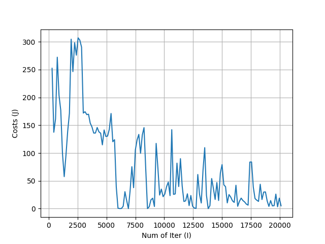
3.3.1. Velocity of 2D-CNN with LSTM Model on some Preprocessor Combinations. TYPO. By Number of Iter(I) there is Number of Samples, during minibatch learning.
Even 2D CNN was enough, I think you could achieve much better with LSTM. The reason here, it's very important to value previous frames to understand acceleration over time. And next feature extraction changes (in our cases Optical Dense Flow) I started with 2D CNN + LSTM and update it to 3D CNN with all power of Keras lib. This Model was one the best on the validation data and speed of learning. Branch with 3D CNN usage TBD
[TBD]
3.4.1. Velocity of 3D-CNN Model.Note. Comparing to previous Plots, this X direction represents epoches over all samples. Since this model was better, we continue training.
Even I had a good result on my validation data, it's will require further review on test data. However, for me it was more a self education task, with great experience on computer vision analyze. This project has a good hints on different AI task, which we could reuse in future.