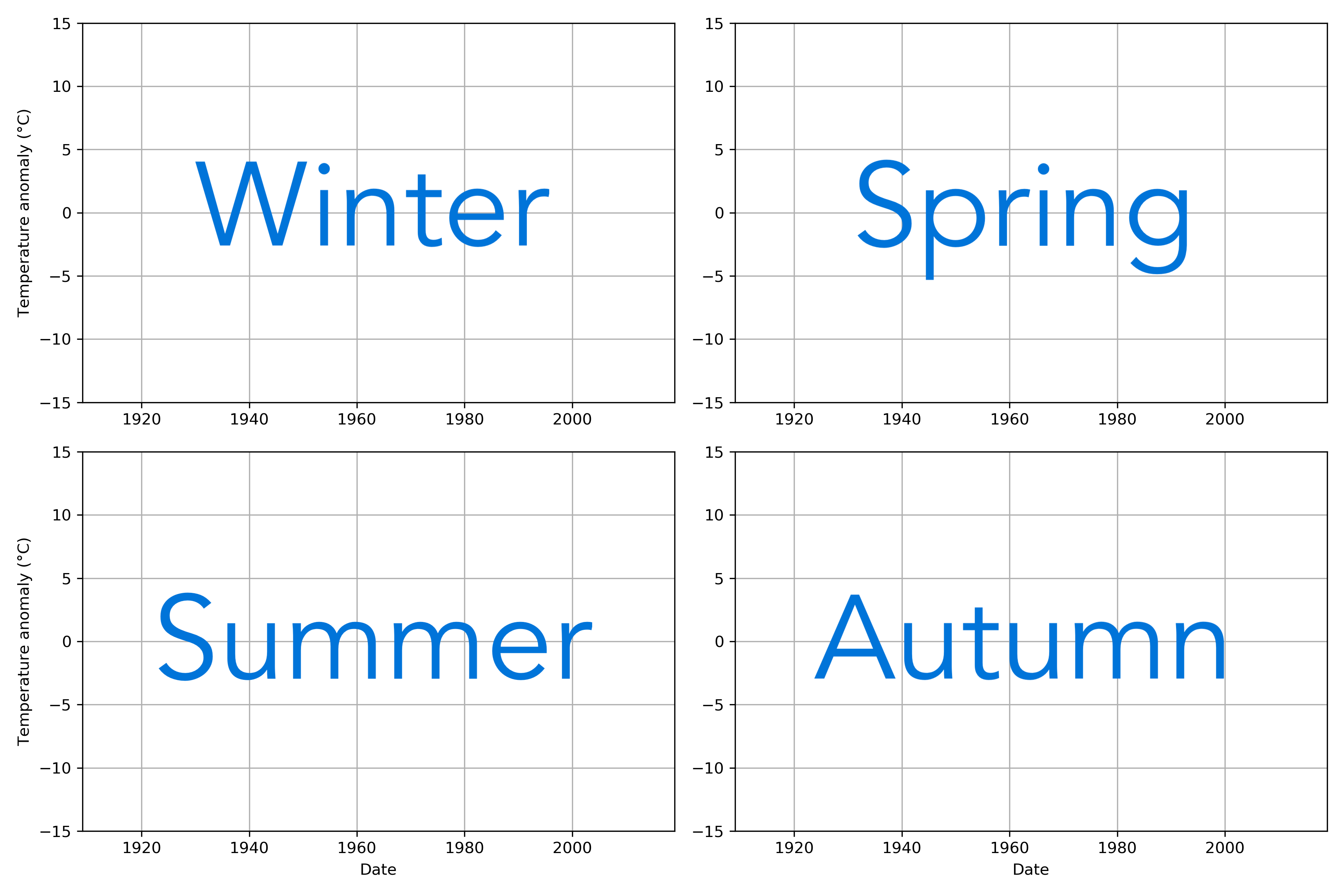
The final exercise in the Geo-Python course involves calculating and plotting seasonal weather anomalies to see how temperatures have changed in different seasons over the past 100+ years. We will be using weather data from the Sodankylä weather station in northern Finland.
As with the earlier exercises in the course you should save your modifications (regularly) in your GitHub repository.
The final exercise is due by 17:00 on November 18, 2022.
- You will be working individually rather than with a partner on this exercise
- We will provide general instructions about what to do, but you will need to determine how you will approach this exercise
- You will have an empty Jupyter notebook and will be responsible for determining how you will use the Markdown and Python cells to perform your analysis
- The exercise is worth 40 points in total
Your task is to create a four-panel plot showing the seasonal temperature anomalies for winter, spring, summer, and autumn for the years 1909-2019. A template for how the final plot should look can be found below.
We have provided a data file for you with daily temperature data from Sodankylä from January 1908 to October 2020. The data was downloaded from the NOAA Global Historical Climate Network database as a text file. The first five lines of the data file can be found below in order for you to see the data format.
STATION           STATION_NAME                                       DATE     TAVG     TMAX     TMIN
----------------- -------------------------------------------------- -------- -------- -------- --------
GHCND:FI000007501                                   SODANKYLA-AWS-FI 19080101 -9999    2        -37
GHCND:FI000007501                                   SODANKYLA-AWS-FI 19080102 -9999    6        -26
GHCND:FI000007501                                   SODANKYLA-AWS-FI 19080103 -9999    7        -27
As you can guess, the temperatures here are given in degrees Fahrenheit and the important columns for you are as follows:
DATE: The date in 'YEARMODA' format, where 'YEAR' is the year using 4 digits, 'MO' is the two-digit month, and 'DA' is the day of the month.TAVG: The average daily temperature in FahrenheitTMAX: The maximum daily temperature in FahrenheitTMIN: The minimum daily temperature in Fahrenheit
Missing data are identified with -9999 and more information about the data can be found on the NOAA website.
You will notice that there are many missing values in the TAVG column. For days where the TAVG values are missing, you can calculate an estimate of the average daily temperature by averaging the TMAX and TMIN values. You may want to do this in a new column. Note don't replace the existing TAVG values with your estimates!
In contrast to earlier exercises in the course, in this exercise we are providing an empty notebook and only general instructions of how to complete the exercise. This is to help us see how much you have learned about programming in Python and to see how you would approach interacting with data using your new skills.
For this exercise you should:
-
Read in the provided data file using pandas and convert missing data to NA values.
-
Fill in the missing values in the
TAVGcolumn with your estimates of the average daily temperature as noted above in the data section. You can then drop any average daily temperatures that are still missing. -
Define and use a function to convert temperatures in Fahrenheit to Celsius.
-
Calculate seasonal average temperatures for each season in every year (e.g., Winter 1909, Spring 1909, Summer 1909, ...)
-
The seasons should include the following months:
- Winter: December, January, February
- Spring: March, April, May
- Summer: June, July, August
- Autumn: September, October, November
-
-
Calculate seasonal average temperatures for the reference period 1951-1980 (e.g., 4 values in total, one for each season)
-
Calculate seasonal temperature anomalies for each year
-
Plot the data as shown in the example above
Note that we also hope to see you use Markdown cells to explain your data analysis, and code comments where needed to explain what your code does.
Grading criteria for the final exercise are available on the course website.
The total number of points you can receive is 40.
