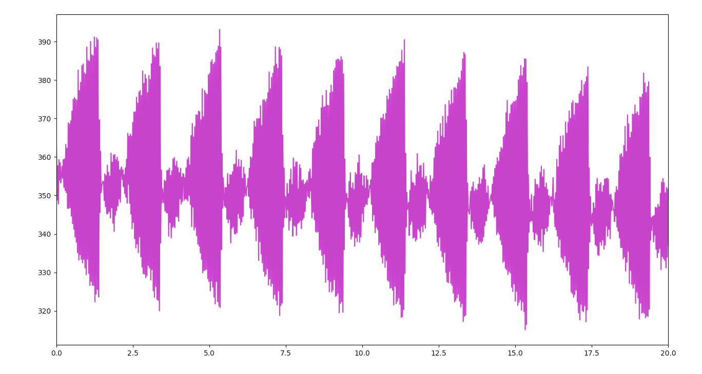
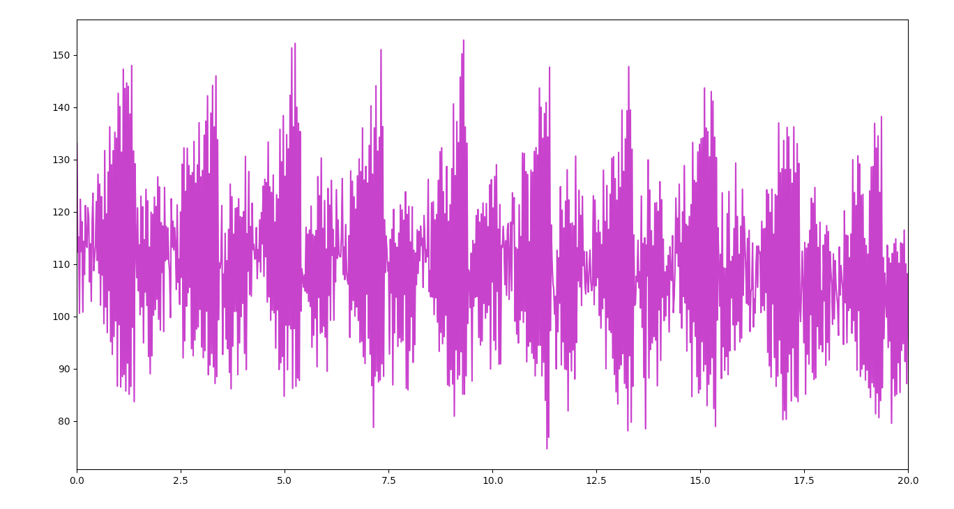
CalciPy: A Python script for processing ratiometric calcium fluorescence data

One of the primary challenges in processing ratiometric data is that the two signals which make up the ratiometric data are actually captured separately, and it is not known which is which. CalciPy processes interlaced calcium fluorescence wavelength data, identifies the proper ratio sequence, and calculates metrics from the resulting signal. See below for more detail. While there is a variety of software for processing calcium fluorescence data, each of them have one or more shortcomings, such as:

Few solutions actually process ratiometric data provided by two wavelengths of light
Some require manual effort to determine the proper ratio and subsequent calculations
Those that can process ratiometric data automatically are limited (e.g. only able to process a single cell line at a time)
Finally, they are not widely available, are closed source, or otherwise proprietary limiting the auditability of the experiments

CalciPy's goal is to enable high throughput, yet customizable, processing of ratiometric calcium fluorescence data, in an open and autidible fashion. It can also serve as a starting point for processing data that is exported from microscopy imaging software, such as Nikon's NIS-Elements. Nikon NIS-Elements is typically used to process images taken from microscopes such as the Nikon Eclipse Ti.

Requirements, Dependencies, and Installation

CalciPy expects that the input file is an Excel file containing ratiometric calcium fluorescent data, which is in the same structure that software packages like Nikon NIS-Elements exports data. See the samples directory for more information.

The script requires Python 2 (v2.7 at least, Python 3 has not been tested yet). Furthermore, the following Python libraries are required and can be installed with Pip.

openpyxl
numpy
scipy
matplotlib
analytic-wfm

Other than that, the script can be run as is when downloaded as a single file.

Running / Command Line Arguments

CalciPy can be run simply by providing the path to the input file as a command line argument. For example:

python calci.py PATH/TO/EXCEL_FILE.xlsx

Additional common examples are as follows. After running the script, you can see the output PDF files and CSV files to determine if you need to add more parameters. If you'd like to output the files to a different directory, use the -O option as follows:

python calci.py -O PATH/TO/OUTPUT_DIRECTORY PATH/TO/EXCEL_FILE.xlsx

If you find that there are more (or fewer) peaks being detected than should be, adjust the look-ahead and delta parameters as below. The look-ahead parameter indicates how far apart (in terms of the number of datapoints - not the amount of time) each peak should be detected. The delta parameter indicates how large of a change in amplitude will be used to identify a peak. It's often best to start by adjusting the look-ahead parameter first, and then adjusting the delta parameter if further refinement is needed.

python calci.py --lookahead 45 --delta .25 -O PATH/TO/OUTPUT_DIRECTORY PATH/TO/EXCEL_FILE.xlsx

Sometimes, you may want to analyze only a portion of a decaying signal. This may be the case if you feel that the signal may be too noisy on the peaks, or if you expect some kind of latency in the signal. You can indicate where the processing of the signal should take place, by percentage of the amplitude. Common paramters in this case are to use 75-25 or 85-10 as follows:

python calci.py --decaystart .85 --decayend .10 --lookahead 45 --delta .25 -O PATH/TO/OUTPUT_DIRECTORY PATH/TO/EXCEL_FILE.xlsx

Curve fitting is, by nature, not exact. When you review the CSV file, you may find that the values for Y0, A, RC, and Tau to be way off your expected results, with very large values for A and very small values (or even negative values) for Y0. The script has the capability to apply some rudementary bounds to the curve fitting process which will limit the outputted values, similar to how Excel's solver can limit output to non-negative values only. This is done with the bounds parameter.

python calci.py --bounds --decaystart .85 --decayend .10 --lookahead 45 --delta .25 -O PATH/TO/OUTPUT_DIRECTORY PATH/TO/EXCEL_FILE.xlsx

If you'd like to view the output graphs interactively, use the show parameter. This is helpful when checking the individual values for peaks and allows you to zoom into each graph. This is facilitated by matplotlib.

python calci.py --show --bounds --decaystart .85 --decayend .10 --lookahead 45 --delta .25 -O PATH/TO/OUTPUT_DIRECTORY PATH/TO/EXCEL_FILE.xlsx

Below is a full list of all the command line arguments that can be used.

usage: calci.py [-h] [-O OUTPUTDIR] [--sheetname SHEETNAME]
                [--sheetnum SHEETNUM] [--column COLUMN]
                [--bgreduce {average,point,none}] [--lookahead LOOKAHEAD]
                [--delta DELTA] [--invert] [--ratioby {time,amplitude}]
                [--decaystart DECAYSTART] [--decayend DECAYEND] [--bounds]
                [--limit LIMIT] [--ymax YMAX] [--ymin YMIN] [--xmax XMAX]
                [--xmin XMIN] [--show] [--verbose]
                filename

Process ratiometric calcium fluorescence decay data.

positional arguments:
  filename              input filename to process

optional arguments:
  -h, --help            show this help message and exit
  -O OUTPUTDIR, --outputdir OUTPUTDIR
                        output files to a directory
  --sheetname SHEETNAME
                        process only a specific worksheet by name (use quotes)
  --sheetnum SHEETNUM   process only a specific worksheet by number
  --column COLUMN       process only a specific cell line column of data
                        (typically 1-10)
  --bgreduce {average,point,none}
                        method for reducing background data
  --lookahead LOOKAHEAD
                        peak detection look-ahead parameter (default=30)
  --delta DELTA         peak detection delta parameter (default=0)
  --invert              invert the waveform (special cases only)
  --ratioby {time,amplitude}
                        method for choosing which ratio to use
  --decaystart DECAYSTART
                        the relative amplitude from the peak where the
                        analysis will start
  --decayend DECAYEND   the relative amplitude from the peak where the
                        analysis will end
  --bounds              bound the solution to non-negative numbers, around the
                        start/end values of the waveform
  --limit LIMIT         limit processing to the first X wavelets (default=0 as
                        disabled)
  --ymax YMAX           output graph Y-axis maximum
  --ymin YMIN           output graph Y-axis minimum
  --xmax XMAX           output graph X-axis maximum
  --xmin XMIN           output graph X-axis minimum
  --show                show the graph (with matplotlib)
  --verbose             print values as they are calculated

Methods

Raw data is exported from software such as Nikon NIS-Elements into an Excel compatible file. See the samples directory for an example data set and format. As mentioned, the two signals which make up the ratiometric data are actually captured separately, represented as interlaced rows in a single dataset, and it is not defined which set of interlaced rows corresponds to what part of the ratio.

To overcome this challenge, the script will analyze different combinations of the data, comparing it with an expected sharp rise and slow(er) decay, typical of calcium fluorescence. The script does this by first iterating over the captured cell lines and subtracting background noise (which should also be captured as the last cell line/column).

Next it de-interlaces the rows to capture the individual signals. At this stage it is not known which signal represents which wavelength of data.

It will divide these two separate signals by eachother to calculate two ratiometric signals, which are purely the inverse of eachother.

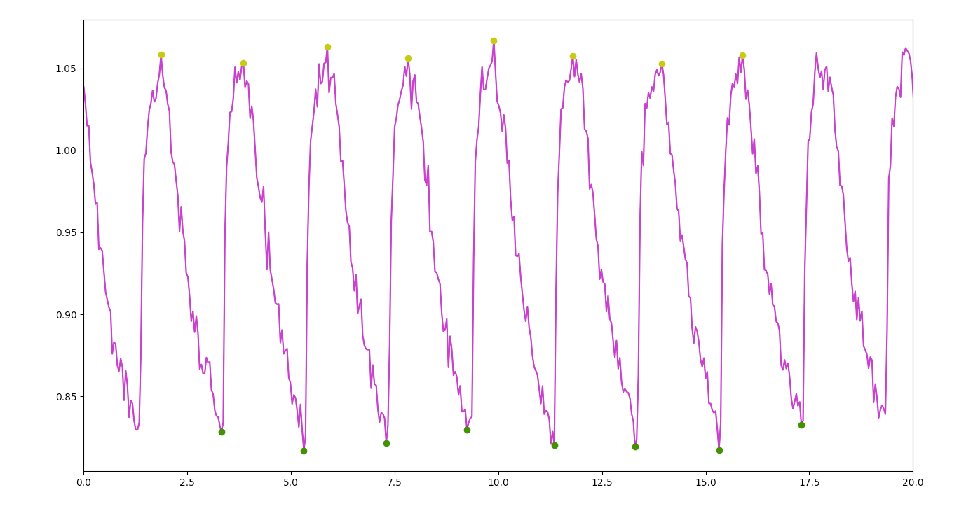
The script then uses look-ahead peak detection to determine local maxima and minima. These detected peaks are used to calculate rise and decay times and identify which combination of rows presents the correct ratio.

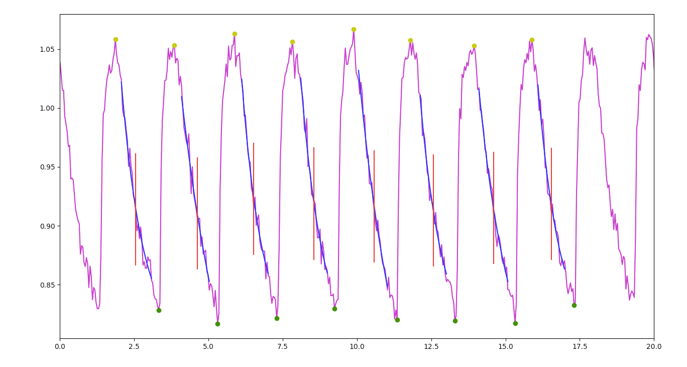
A centered window moving average is applied to the decay data only (each individual set of maximum to minimum), slightly smoothing the signal to obtain more consistent initial values for curve fitting. Python’s curve fitting functions found in SciPy are then used with an exponential decay function to establish the signal’s parameters, most significantly the decay rate (which can also be used to calculate Tau).

The original signal, peaks, fitted curve results, and marker for the position of Tau are then plotted and exported as PDFs for easy visual review.

In addition, calculated results for rate constant, Tau, decay time, amplitude, diastolic, beat rate, beat variation, and velocity are all outputted to a comma separated value text file (CSV) for further analysis. The script can be configured with different peak detection look-ahead windows, amplitude windows, background noise reduction, smoothing filters and more, and has shown consistent results even when run against noisy or arrhythmic signals.

Caveats and Troubleshooting

This software comes without any warrantee or guarantee. While it has shown to provide consistent results, even when run against noisy or arrhythmic signals, verification is still encouraged. Below are some notes of what to look out for during the verification process.

Different versions of Python, with different versions of scipy, and even different computers may output different curve fit parameters for the same input data. In that case, your own judgement should be used to determine if the output is close enough to be considered accurate.
Use the --show option or view the outputted PDF files to visually check the results
When using the --show option, the outputed PDF files will actually come out at a lower resolution. This is because the same graph is used for the screen and PDF and the default window resolution for matplotlib is used when outputting to screen.
You may notice that some min/max peaks at the start or end of the signal do not get detected. This is normal for two reasons. First, a wavelet not be complete at the beginning or end of the signal, and the peak detection algorithm may ignore it. Second, as the script was written with calcium fluorescence decay as a primary use case, if a min peak is detected at the beginning of a signal or a max peak at the end of a signal, they will be removed as to only focus on complete decaying wavelets.
Data that is extremely noisy may still pose problems with analysis. You should expect this if you are unable to see visible peaks in the data manually.
If you see that the larger peaks are detected along side very small peaks, test out different --lookahead and --delta parameters
The same should be true for if the script is not able to provide the correct ratio. To force the script to invert the ratios, use the --invert option.
Environmental factors such as temperature or humidity may cause high precision microscopy instruments to lose focus or become otherwise uncalibrated over time. Use the --limit option to only process a subset of the data.
Some code is not implemented in the most performant or elegant manner possible. One reason for this is so that is a little easier for those who are new to Python and haven't learned all its powerful capabilities with handling data.
As previously mentioned, this script has not been tested with Python 3.

Special Thanks

I'd like to thank the following people at the Stanford Cardiovascular Institute who provided data, feedback, and guidance while this script was being written.

Rajani Shrestha, Research Associate
Timon Seeger, MD / Postdoctoral Fellow
Chi Keung Lam, PhD
Ioannis Karakikes, PhD
Isaac Perea-Gil, PhD