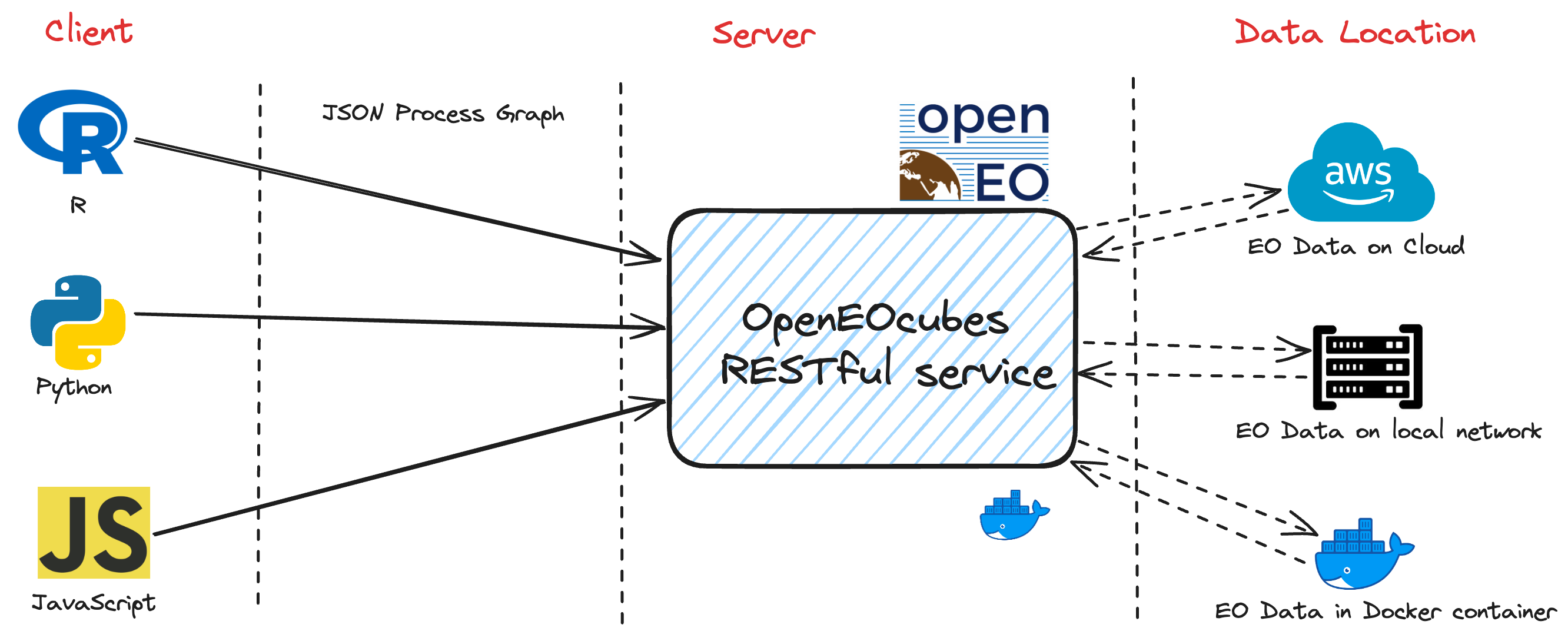
The service integrates STAC API (using Rstac package), the OpenEO standardized API, and data cubes concepts (using gdalcubes R package) to be a lightweight platform to enable analysis of time series satellite images via OpenEO Compliant RESTful endpoints using R-Client. It also supports users to run their custom R functions.
The service tries to improve on the limitations of established EO data management platforms like Google Earth Engine and Sentinel Hub by supporting:
- Reproducibility of Science
- Extensibility
- Infrastructure Replicability
- Open Governance
- No Need for User Management
- User-Defined R Functions
- Flexibility - Custom CRS, and Quick Resampling of Massive EO Data
After processing the data , one can download and explore on open source tools like QGIS, R, Python, etc.
Geospatial Machine Learning APIs for time-series EO Data:
- ML APIs e.g. Random Forest, SVM, XGBoost, etc.
- DL APIs e.g. TempCNN, ResNet, etc.
Currently PoC is being worked on at this reposity on the Open Earth Monitor Cyberinfrastructure EU funded project.
Assuming you have Docker installed. This is the easiest approach. You can get a hosted Docker image of the platform on DockerHub https://hub.docker.com/r/brianpondi/openeocubes
It is highly recommended to deploy the service on an AWS EC2 machine that is in us-west-2 region (Oregon) as that is the data centre where the Earth Observation(EO) datasets found in AWS STAC search are stored. This enables the processing of EO data from the source so that the network latency between the platform and data is as low as possible hence cheaper. You can expose port 8000 of the EC2 instance to deploy and communicate with the service.
docker run -p 8000:8000 --env AWSHOST=<AWS-IPv4-ADDRESS> brianpondi/openeocubesFor light tasks and processes you can host the service on pc and therefore you don't need AWS IPv4 Address
docker run -p 8000:8000 brianpondi/openeocubesIf you want to change the source code then this approach is recommended. You first need to clone the repository via this command:
git clone https://github.com/PondiB/openeocubes.gitthen you can change to that directory
cd openeocubesRun it :
docker-compose upRun in detached mode :
docker-compose up -dShutting it down:
docker-compose downForce restart and rebuild:
docker-compose up --build --force-recreate --no-deps -dIf there are new changes on the images or Dockerfiles:
docker-compose build --no-cache && docker-compose up
While developing, you can skip rebuilding the docker container everytime. Instead you can run the server locally. Just run "Rscript startLocal.R" inside this directory.
This will compile this Repository as a R Package and start the server.
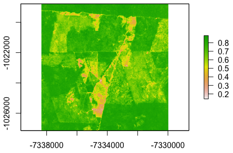
Using openeo client version 1.3.0, the R scripts provided below calculate a 1-year period NDVI in a section of Amazonia in Brazil.
library(openeo)

# connect  to the back-end when deployed locally
 con = connect("http://localhost:8000")
# connect  to the back-end when deployed on aws
# con = connect("http://<AWS-IPv4-ADDRESS>:8000")

# basic login with default params
login(user = "user",
      password = "password")

# get the collection list
collections = list_collections()

# to check description of a collection
collections$`sentinel-s2-l2a-cogs`$description

# Check that required processes are available.
processes = list_processes()

# to check specific process e.g. ndvi
describe_process(processes$ndvi)

# get the process collection to use the predefined processes of the back-end
p = processes()

# load the initial data collection and limit the amount of data loaded
datacube_init = p$load_collection(id = "sentinel-s2-l2a-cogs",
                                spatial_extent = list(west=-7338335,
                                                      south=-1027138,
                                                      east=-7329987,
                                                      north=-1018790),
                                                      crs = 3857,
                                temporal_extent = c("2021-05-01", "2022-06-30"))

# filter the data cube for the desired bands
datacube_filtered = p$filter_bands(data = datacube_init, bands = c("B04", "B08"))

# aggregate data cube to a year
datacube_agg = p$aggregate_temporal_period(data = datacube_filtered, period = "year", reducer = "median")

# ndvi calculation
datacube_ndvi = p$ndvi(data = datacube_agg, red = "B04", nir = "B08")

# supported formats
formats = list_file_formats()

# save as GeoTiff or NetCDF
result = p$save_result(data = datacube_ndvi, format = formats$output$GTiff)

# Process and download data synchronously
start.time <- Sys.time()
compute_result(graph = result, output_file = "amazonia_2022_ndvi.tif")
end.time <- Sys.time()
time.taken <- end.time - start.time
time.taken
print("End of processes")
Visualization of the output from the above process:
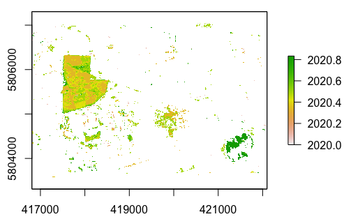
Using openeo client version 1.3.0, the R scripts provided below has a user-defined function that uses bfast library to monitor changes on time series of Sentinel-2 imagery from 2016 to 2020. The study area is the region around the new Berlin-Brandenburg Tesla Gigafactory. You can run the code on your R-studio.
library(openeo)

# connect  to the back-end when deployed locally
 con = connect("http://localhost:8000")
# connect  to the back-end when deployed on aws
#con = connect("http://<AWS-IPv4-ADDRESS>:8000")

# basic login with default params
login(user = "user",
      password = "password")

# get the collection list
collections = list_collections()

# to check description of a collection
collections$`sentinel-s2-l2a-cogs`$description

# check that required processes are available.
processes = list_processes()

# to check specific process e.g. filter_bands
describe_process(processes$filter_bands)

# get the process collection to use the predefined processes of the back-end
p = processes()

# load the initial data collection and limit the amount of data loaded
datacube_init = p$load_collection(id = "sentinel-s2-l2a-cogs",
                                  spatial_extent = list(west=416812.2,
                                                        south=5803577.5,
                                                        east=422094.8,
                                                        north=5807036.1),
                                                        crs = 32633,
                                  temporal_extent = c("2016-01-01", "2020-12-31"))

# filter the data cube for the desired bands
datacube_filtered = p$filter_bands(data = datacube_init,
                                          bands = c("B04", "B08"))
# aggregate data cube to monthly
datacube_agg = p$aggregate_temporal_period(data = datacube_filtered,
                            period = "month", reducer = "median")

# user defined R function - bfast change detection method
change_detection = 'function(x) {
  knr <- exp(-((x["B08",]/10000)-(x["B04",]/10000))^2/(2))
  kndvi <- (1-knr) / (1+knr)
  if (all(is.na(kndvi))) {
    return(c(NA,NA))
  }
    kndvi_ts = ts(kndvi, start = c(2016, 1), frequency = 12)
    library(bfast)
    tryCatch({
        result = bfastmonitor(kndvi_ts, start = c(2020,1), level = 0.01)
        return(c(result$breakpoint, result$magnitude))
      }, error = function(x) {
        return(c(NA,NA))
      })
  }'

# run udf
datacube_udf = p$run_udf(data = datacube_agg, udf = change_detection, context =  c("change_date", "change_magnitude"))

# supported formats
formats = list_file_formats()

# save as GeoTiff or NetCDF
result = p$save_result(data = datacube_udf, format = formats$output$NetCDF)

# Process and download data synchronously
start.time <- Sys.time()
compute_result(graph = result, output_file = "detected_changes.nc")
end.time <- Sys.time()
time.taken <- end.time - start.time
time.taken
print("End of processes")
Visualization of the output from the above process:


