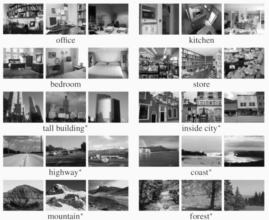
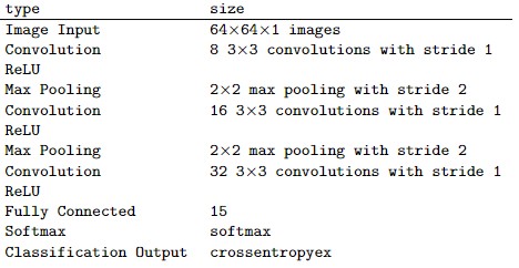
Problem statement Computer vision is a field of artificial intelligence that enables computers and systems to derive meaningful information from digital images, videos and other visual inputs, and based on those inputs, it can take action. The aim of this project is to implement an image classifier based on convolu- tional neural networks. Starting by implementing a simple shallow network and then refining it until a pre-trained ResNet18 is implemented, showing at each step how the accuracy of the model improves. The provided dataset (from [Lazebnik et al., 2006]) contains 15 categories.
Convolutional neural networks have three main types of layers, which are:
The convolutional layer is the core building block of a CNN, and it is where the majority of computation occurs. It requires a few components, which are input data, a filter, and a feature map. Let’s assume that the input will be a color image, this means that the input will have three dimensions: height, width, and depth, which correspond to RGB in an image. We also have a feature detector, also known as a kernel or a filter, which will move across the fields of the image, checking if the feature is present. This process is known as a convolution. The filter is applied to an area of the image, and a dot product is calculated between the input pixels and the filter. This dot product is then fed into an output array. Afterwards, the filter shifts by a stride, repeating the process until the kernel has crossed the entire image. The final output from the series of dot products from the input and the filter is known as a feature map, activation map, or a convolved feature. There are three hyperparameters which affect the volume size of the output that need to be set before the training of the neural network begins. These include:
- The number of filters affects the depth of the output. 2
- Stride is the distance, or number of pixels, that the kernel moves over the input matrix.
- Padding, this sets all elements that fall outside of the input matrix, pro- ducing a larger or equally sized output. There are three types of padding: Valid padding, Same padding and Full padding.
After each convolution operation, it is applies a transformation to the feature map (ReLu, Sigmoid, Than, ...), introducing nonlinearity to the model. The convolutional layer converts the image into numerical values, allowing the neural network to interpret and extract relevant patterns.
The pooling operation performs a filter on the input, but the difference is that this filter has no weights. Instead, it applies an aggregation function to the values within the considered field, populating the output array. There are two main types of pooling:
- Max pooling: As the filter moves across the input, it selects the pixel with the maximum value to send to the output array.
- Average pooling: As the filter moves across the input, it calculates the average value within the considered field to send to the output array.
It has a number of benefits to the CNN. They help to reduce complexity, improve efficiency, and limit risk of overfitting.
The name of the fully connected layer describes itself appropriately. As already mentioned, in partially connected layers, the pixel values of the input image are not directly connected to the output layer. In the fully connected layer, however, each node of the output layer connects directly to a node of the previous layer. This layer performs the task of classification based on the features extracted through the previous layers and their various filters. While convolutional and pooling layers tend to use activation functions, FC layers usually exploit a softmax activation function to classify inputs appropriately, producing a probability of 0 to 1.
A proper initialization method should avoid reducing or magnifying the magni- tudes of input signals exponentially. He initialization refers to the first author in the paper “Delving Deep into Rectifiers: Surpassing Human-Level Performance on ImageNet Classification”. This method is similar to Xavier initialization, with the factor multiplied by two. In this method, the weights are initialized keeping in mind the size of the previous layer which helps in attaining a global minimum of the cost function faster and more efficiently.The weights are still random but differ in range depending on the size of the previous layer of neurons. This provides a controlled initialization hence the faster and more efficient gradient descent. He initialization initializes the bias vectors of a neural network to 0 and the weights to random numbers drawn from a Gaussian distribution where the mean is 0 and the std √︂2 nl, where nlis the dimension of the previous layer.
The provided dataset from [Lazebnik et al., 2006], contains 15 categories (office, kitchen, living room, bedroom, store, industrial, tall building, inside city, street, highway, coast, open country, mountain, forest, suburb), and is already divided in training set and test set. So we divided the training set provided into 85% for the actual training set and 15% to be used as the validation set.
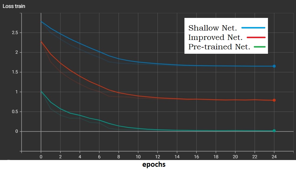
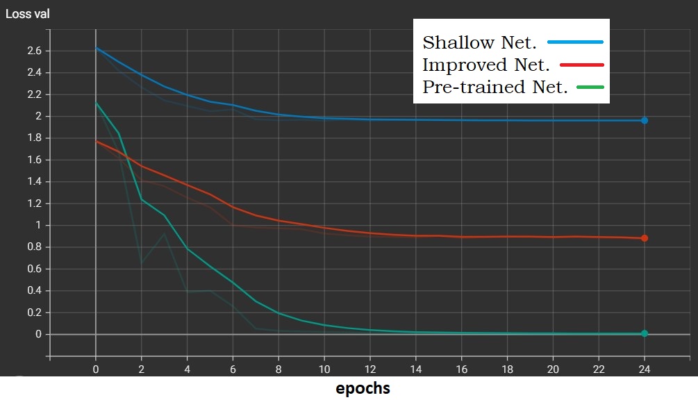
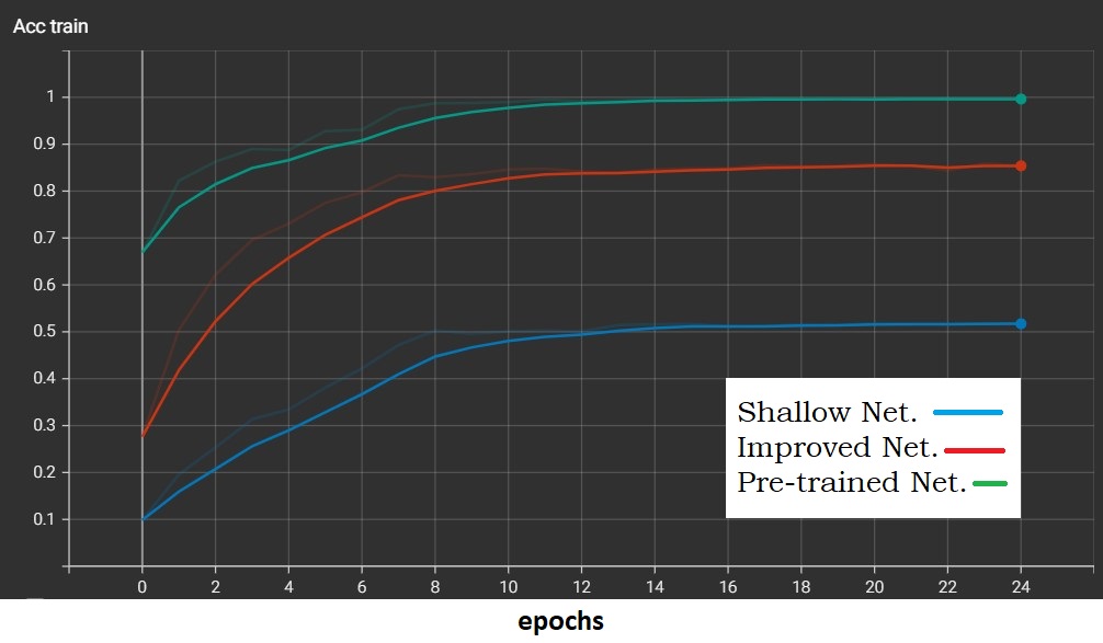
For the following results, in all networks, a mini-batch of size 32 was used and the initial weights were initialised using He Normal Initialisation (see above). Also, a cross-entropy loss was used to define the cost function. Stopping criteria: An early stop is used as a stopping criterion, whereby when an increase in the validation error is observed or this stabilises, training is interrupted and the best parameters are stored and returned. Learning rate Schedules: Learning rate schedules seek to adjust the learning rate during training by reducing the learning rate according to a pre- defined schedule. We use a exponential decay.
Since the input image is 64×64, the images had to be resized in order to feed them to the network. Anisotropic scaling was implemented. Also, a gray scaling process of converting an image from the color spaces RGB (3 channels) to shades of gray (1 channel) was applied. As optimiser, we used a Stochastic Gradient Descent.
For this Networks data augmentation was used. In particular, it was applied randomly, only to the training set, a vertical and horizontal Flip. This tecnique make the dataset more robust, and improve the performance. We also introduced a Batch Normalization before the activation functions, with the aim of reducing the internal covariance shift and making the model more robust. Finally we add some dropout layer to improve regularization. As optimiser, we used Adam optimizer.
In finetuning, we start with a pre-trained model and update all of the model’s parameters for our new task, in essence retraining the whole model. In our case a pre-trained ResNet18 was used. Since ResNet18 takes images of size 256x256 as input, we had to resize our images before feeding the training. Also in this case we used the Augmented dataset. The workflow is:
- Initialize the pretrained model
- Reshape the final layer(s) to have the same number of outputs as the number of classes in the new dataset
- Define for the optimization algorithm which parameters we want to update during training
- Run the training step
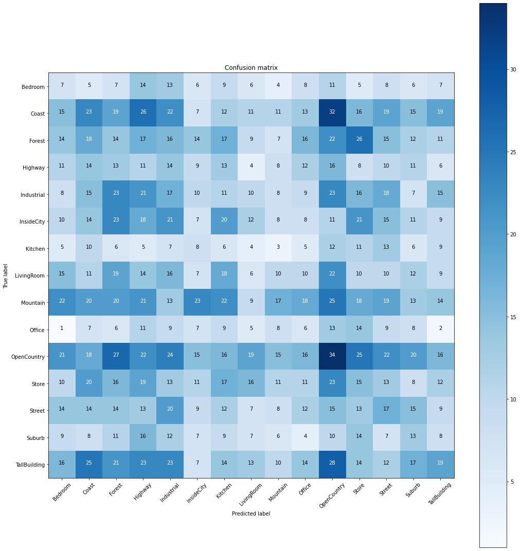
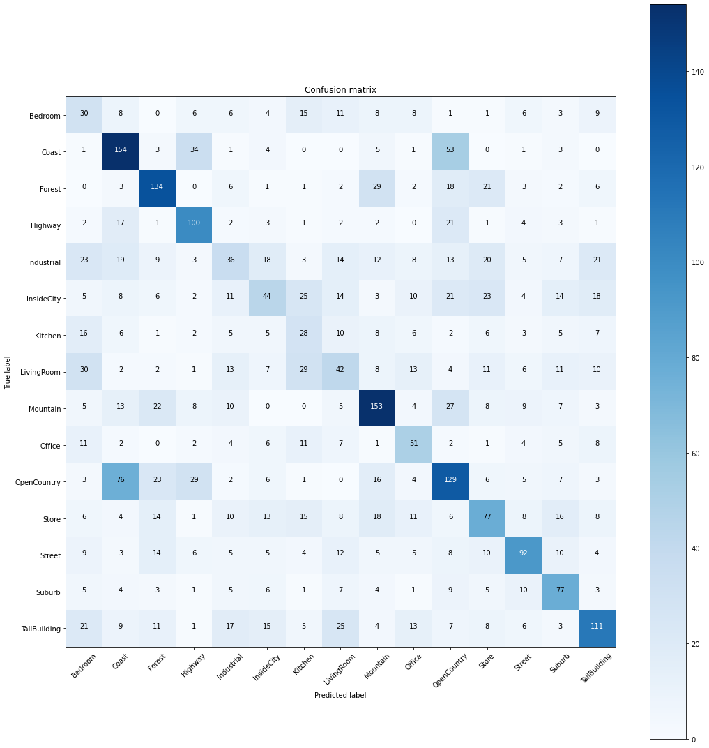
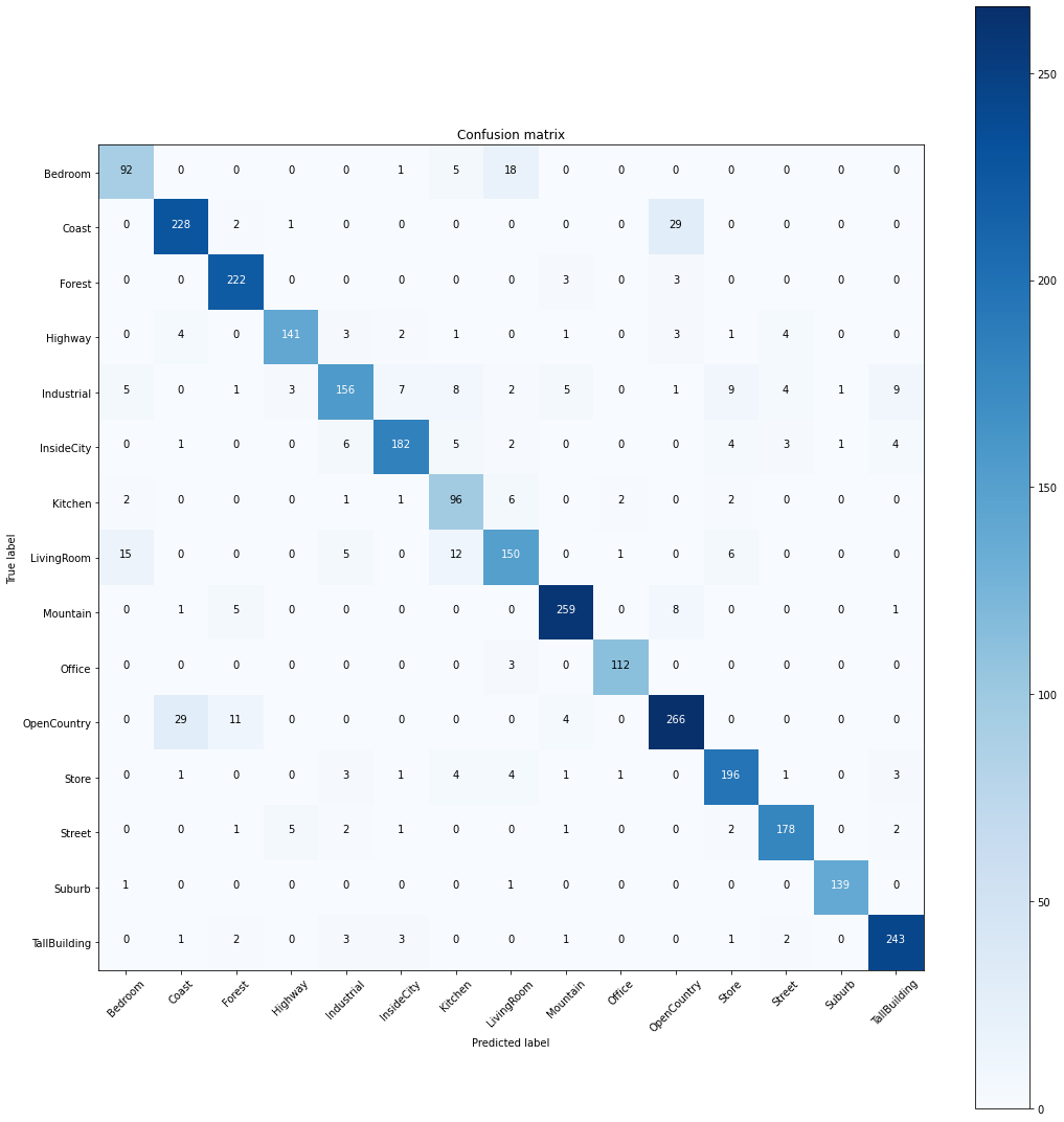
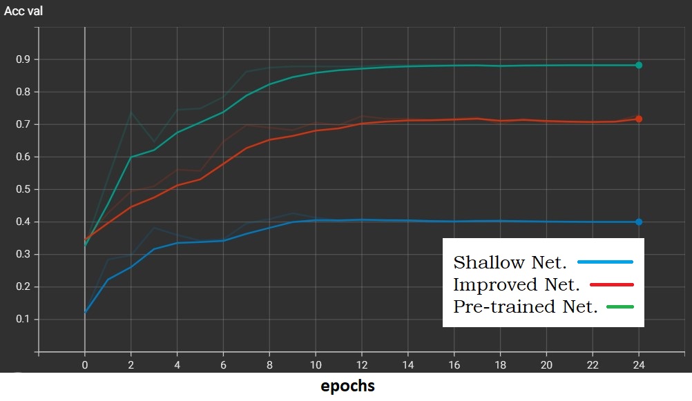
According to the stop criteria, the best parameters are stored after the training is stopped. In the following the best result for validation accuracy during training:
- Shallow Network: Best val Acc: 0.426667
- Improved Network: Best val Acc: 0.729412
- Pre-trained Network: Best val Acc: 0.882353
