easyplot: A matplotlib wrapper written in Python to enable fast and easy creation of reusable plots.
The EasyPlot module provides a thin wrapper to matplotlib, enabling fast and easy generation of beautiful, annotated plots with minimal code. It also enables the reuse of EasyPlot instances to generate new plots that maintain state from previous plots allowing for quick and easy generation of multiple plots of a similar type. EasyPlot supports all commonly used plot parameters and allows access to the underlying figure and axes instances to allow the user to further customize the generated plots if necessary.
I'd love to hear your comments and/or suggestions. You can get in touch with me via [twitter](https://twitter.com/hamsterhuey), [email](mailto:sudeepmandal@gmail.com) or [google+](https://plus.google.com/u/0/105292596991480463202/)
This document is also viewable online as an IPython Notebook:
http://nbviewer.ipython.org/github/HamsterHuey/easyplot/blob/master/docs/easyplot_docs.ipynb
- Requirements
- Installation
- Motivation and Background
- Features
- Documentation
- Usage and Examples
- Advanced plotting
- Python 2.7.2+
- matplotlib
Use of the IPython shell is strongly recommended with
this library (and matplotlib plotting in general). The %matplotlib magic
command in IPython (or starting IPython using ipython --matplotlib) implements
a number of backend tweaks to enable robust, interactive plotting using
matplotlib.
You can use the following commands to install EasyPlot:
pip install easyplot
or
easy_install easyplot
Alternatively, you could download the package manually from the Python Package Index: https://pypi.python.org/pypi/EasyPlot, unzip it, navigate into the package, and use the command:
python setup.py install
or
pip install .
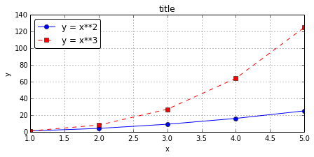
Setting up aesthetically pleasing plots with plot titles, axes labels, etc requires several lines of boilerplate code in vanilla matplotlib. As an example, creating a basic plot in matplotlib requires the following lines of code:
fig, ax = plt.subplots()
ax.plot(x, x**2, 'b-o', label="y = x**2")
ax.plot(x, x**3, 'r--s', label="y = x**3")
ax.legend(loc='best')
ax.grid()
ax.set_xlabel('x')
ax.set_ylabel('y')
ax.set_title('title')
Pylab alleviates some of this, but still requires calls to a number of different functions that are commonly used (such as xlabel, xlim, etc.). More complicated plots can require several more lines of code. Typing all this code every time to generate plots gets tedious very quickly. This situation is further exacerbated when working in an IPython Notebook where all plots typically need to be labeled, annotated and looking their best. Having several lines of code preceeding every plot in a notebook can break the flow of the document and distract from the code/concepts being presented by the author. Furthermore, oftentimes, plots with similar labels and formatting need to be generated repeatedly with different datasets. Generating these sets of plots would require retyping these same lines of boilerplate code across different sections of your code/notebook.
Easyplot is my attempt to address these issues and make generating quick,
pleasant looking, annotated plots a bit easier. In keeping with DRY
philosophy, easyplot
enables the creation of an EasyPlot object that maintains state information of
all plot parameters passed to it in order to generate a plot. This can then be
easily reused to generate new plots with the user only having to supply any
additional plot parameters, or those parameters he or she wishes to override
from the previous plot.
Easyplot supports a large number of standard plot parameters that most users
typically deal with when plotting in matplotlib. Additionally, it provides
methods to access the figure and axes instance for the latest plot, enabling
users to perform more custom plot modifications that are not directly supported
by easyplot. It also supports interactive plotting where additional plot
parameters can be passed to the current plot using the update_plot method. The
plot above can be generated using easyplot as follows:
eplot = EasyPlot(x, x**2, 'b-o', label='y = x**2', showlegend=True,
                 xlabel='x', ylabel='y', title='title', grid='on')
eplot.add_plot(x, x**3, 'r--s', label='y = x**3')
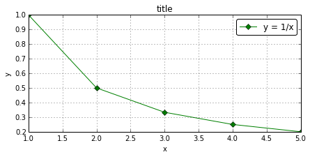
Along with the reduced typing, easyplot enables the consolidation and passing of all plot parameters into a single plot call. This is already quite handy, but the real benefit is evident when one needs to generate a new plot with the same plot parameters (such as axis labels and title) but with new data:
eplot.new_plot(x, 1/x, 'g-D', label='y = 1/x')EasyPlot also provides an iter_plot() method that iterates through x, y data
and plot parameters that are provided in a list or dictionary format to
automatically generate an annotated, multi-line plot with a single statement:
eplot = EasyPlot(xlabel=r'$x$', ylabel='$y$', fontsize=16,
                 colorcycle=["#66c2a5","#fc8d62","#8da0cb"], figsize=(8,5))
eplot.iter_plot(x, y_dict, linestyle=linestyle_dict, marker=marker_dict,
label=labels_dict, linewidth=3, ms=10, showlegend=True, grid='on')- Access to a large number of the most used matplotlib plot parameters under a unified wrapper class
- Plot parameter aliases supported. Can be extended by user for arbitrary alias definitions for various plot parameters
- Ability to use
EasyPlotobjects as templates to rapidly generate annotated plots of a similar type iter_plot()method to easily iterate through x, y datasets and plot multiple plots with a single method call- Draggable legend when using GUI backends (eg: qt, wx, etc.)
- Provides access to underlying figure, axes and line2D objects for advanced plot customization
EasyPlot consists of an EasyPlot class to create EasyPlot() objects in order
to generate matplotlib plots. The object constructor allows for passing all
commonly used plot parameters (such as xlabel, ylabel, title,
markersize, linewidth, etc.) and the x, y data and an optional format
string as arguments in order to generate an annotated plot via a single
statement such as:
fftplot = EasyPlot(freq, amplitude, 'g-o', markersize=9, linewidth=3,
                xlabel='Frequency (Hz)', ylabel='Amplitude', label='FFT Data', showlegend=True)
If no x, y data is provided to the EasyPlot constuctor, creation of a
figure and axes instance for the EasyPlot object is deferred and the plot
parameters that are passed to the constructor are used to initialize the
EasyPlot object.
Apart from the usual plot parameters, EasyPlot constructor also takes the
following special keyword arguments:
fig : an optional reference to a figure object supplied by the user
ax : an optional reference to an axes object (linked to fig) to use for
displaying the plots. The subplots example demonstrates the use of
fig and ax plot parameters for custom plotting routines
figsize : the size of the plot figure
showlegend : set to True or False to display the plot legend
The EasyPlot object also retains state information of most plot parameters
passed to it, thus allowing the object to be reused as a template for generating
new plots with similar formatting/labeling. The only parameters whose values are
not persistent are color, marker, linestyle and label as they are
assumed to be unique to a single plot.
EasyPlot objects also provide access to their figure, axes and Line2D
instances via the get_figure(), get_axes() methods and line_list instance
variable respectively.
The main instance methods for EasyPlot objects are:
add_plot(*args, **kwargs) : This is the main instance method to add additional
plots and plot parameters to an existing plot. *args is a variable length
argument, allowing for x, y pairs with an optional format string of the form
'b-o'. The optional format string is a shorthand for specifying the plot color
, linestyle and marker type. The [matplotlib docs]
(http://matplotlib.org/1.3.1/api/pyplot_api.html#matplotlib.pyplot.plot) provide
more information regarding the format string notation. **kwargs are a list of
named plot parameters as explained in the next section.
update_plot(**kwargs) : Instance method to update plot parameters only
(example: xlabel, title, etc.). This method is typically only useful when
plotting interactively using an interactive matplotlib backend.
new_plot(*args, **kwargs) : Create a new plot using the plot parameters of the
existing EasyPlot instance as a template (i.e., plot parameter settings carry
over from the EasyPlot instance to the new plot)
iter_plot(x, y, mode='dict', **kwargs) : This method can be used to plot
multiple line/scatter plots with a single statement as long as x, y, and any
relevant plot parameters that change for each plot are passed in as either a
dictionary with a common set of keys (mode='dict') or a set of lists/arrays
corresponding to each data set to be plotted (mode='array').
autoscale(enable=True, axis='both', tight=None) : Set autoscale options for
x, y or both axes
grid(**kwargs) : Equivalent to matplotlib axes.grid() method and accepts same
set of keyword arguments. Enables more custom control over the plot grid.
get_figure() : Returns reference to the Figure object for the instance
get_axes() : Returns reference to the axes object for the instance
redraw() : Forces a redraw of the plot canvas. Must be used if custom
modifications are made to the plot external to easyplot via direct access to the
figure and axes handles. Note: redraw() is only supported when plotting in
interactive mode (i.e. plt.isinteractive() == True).
set_fontsize(font_size) : Modify global setting for plot font-size
The main instance variables for EasyPlot objects are:
self.kwargs : A dictionary containing a list of all existing plot parameters
for an EasyPlot object. The user should not modify this directly. This
variable should be accessed in a read-only fashion for the purposes of examining
the state of an EasyPlot object.
self.line_list : A list of [Line2D](http://matplotlib.org/1.3.1/api/artist_a
pi.html#matplotlib.lines.Line2D) items corresponding to all plots of the
EasyPlot object. These can be manipulated using standard matplotlib methods
outside of easyplot for advaced plotting.
Plot Parameters:
----------------
fig : figure instance for drawing plots
ax : axes instance for drawing plots (If user wants to supply axes,
     figure externally, both ax and fig must be supplied together)
figSize : tuple of integers ~ width & height in inches
label : Label for line plot as determined by *args, string
color / c : Color of line plot, overrides format string in *args if
            supplied. Accepts any valid matplotlib color
linewidth / lw : Plot linewidth
linestyle / ls : Plot linestyle ['-','--','-.',':','None',' ','']
marker : '+', 'o', '*', 's', 'D', ',', '.', '<', '>', '^', '1', '2'
markerfacecolor / mfc : Face color of marker
markeredgewidth / mew :
markeredgecolor / mec :
markersize / ms : Size of markers
markevery / mev : Mark every Nth marker
                  [None|integer|(startind, stride)]
alpha : Opacity of line plot (0 - 1.0), default = 1.0
title : Plot title, string
xlabel : X-axis label, string
ylabel : Y-axis label, string
xlim : X-axis limits - tuple. eg: xlim=(0,10). Set to None for auto
ylim : Y-axis limits - tuple. eg: ylim=(0,10). Set to None for auto
xscale : Set x axis scale ['linear'|'log'|'symlog']
yscale : Set y axis scale ['linear'|'log'|'symlog']
    Only supports basic xscale/yscale functionality. Use
    get_axes().set_xscale() if further customization is required
grid : Display axes grid. ['on'|'off']. See grid() for more options
colorcycle / cs: Set plot colorcycle to list of valid matplotlib
                 colors
fontsize : Global fontsize for all plots

Legend Parameters:
------------------
showlegend : set to True to display legend
fancybox : True by default. Enables rounded corners for legend box
framealpha : Legend box opacity (0 - 1.0), default = 1.0
loc : Location of legend box in plot, default = 'best'
numpoints : number of markers in legend, default = 1.0
ncol : number of columns for legend. default is 1
markerscale : The relative size of legend markers vs. original.
              If None, use rc settings.
mode : if mode is “expand”, the legend will be horizontally
       expanded to fill the axes area (or bbox_to_anchor)
bbox_to_anchor : The bbox that the legend will be anchored. Tuple of
                 2 or 4 floats
It is strongly recommended that EasyPlot be used in a Python/IPython shell
with interactive matplotlib plotting turned on (matplotlib.pyplot.ion() turns
this on). This provides the maximum flexibility when plotting with EasyPlot
and also makes it easier to learn and understand the use of this matplotlib
wrapper. In the case of non-interactive plotting, the blocking nature of
plt.show() prevents dynamic modification and further additions to an existing
plot. This issue can be partially alleviated by the plt.show(block=False)
method call (this is experimental in Matplotlib).
Note that if non-interactive plotting is the default, the user must call
plt.show() after setting up the plot as desired using EasyPlot. add_plot()
method calls on the EasyPlot instance are not supported after the figure is
closed in non-interactive mode, and the redraw() instance method is also not
supported in this mode (user can call plt.draw() instead)
# Import modules and setup
%matplotlib inline
import matplotlib.pyplot as plt
import numpy as np
from easyplot import EasyPlot

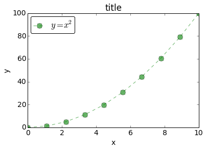
x = np.linspace(0, 10, 10)eplot = EasyPlot(x, x**2, 'g--o', label=r"$y = x^2$", showlegend=True, xlabel='x',
ylabel='y', title='title', fontsize=14, markersize=10, alpha=0.6)#Note the use of plot parameter aliases and the figsize parameter
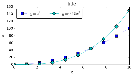
eplot = EasyPlot(x, x**2, label=r"$y = x^2$", figsize=(8,4), showlegend=True,
ncol=2, ms=10, ls=':', markeredgewidth=1.5, xlabel='x',
ylabel='y', title='title', color='b', marker='s')
eplot.add_plot(x, 0.15*x**3, label='$y = 0.15x^3$', c='c', ls='-', marker='D')The previous example defined an EasyPlot object eplot with various plot
parameters set - xlabel, ylabel, title, alpha, ncol, markersize and
markeredgewidth . We can examine the current set plot parameters for an
EasyPlot object by accessing its kwargs instance variable
#Examine set plot parameters for eplot
eplot.kwargs

{'ax': <matplotlib.axes.AxesSubplot at 0x4485650>,
 'dpi': 80,
 'fancybox': True,
 'fig': <matplotlib.figure.Figure at 0x446d8f0>,
 'figsize': (8, 4),
 'loc': 'best',
 'markeredgewidth': 1.5,
 'markersize': 10,
 'ncol': 2,
 'numpoints': 1,
 'showlegend': True,
 'title': 'title',
 'xlabel': 'x',
 'ylabel': 'y'}
Note that certain plot parameters such as linestyle, marker, label and
color are considered unique parameters and do not carry over from one plot
to another as they are typically unique to a specific plot.
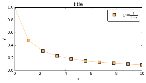
It is easy to use eplot as a template to generate a new plot:
eplot.new_plot(x, 1/(1+x), '-s', label=r"$y = \frac{1}{1+x}$", c='#fdb462')
# Note that the plot reuses the axis labels, title and marker
# formatting from the previous eplot templateEasyPlot objects have an autoscale() instance method that can be called on the
instance to reset the xlim and ylim properties to None and autoscale the
axes. The method signature is listed below along with the default parameter
values.
def autoscale(self, enable=True, axis='both', tight=None):
    """Autoscale the axis view to the data (toggle).

    Convenience method for simple axis view autoscaling. It turns
    autoscaling on or off, and then, if autoscaling for either axis is on,
    it performs the autoscaling on the specified axis or axes.

    Arguments
    =========
    enable: [True | False | None]
    axis: ['x' | 'y' | 'both']
    tight: [True | False | None]
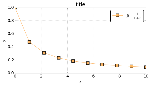
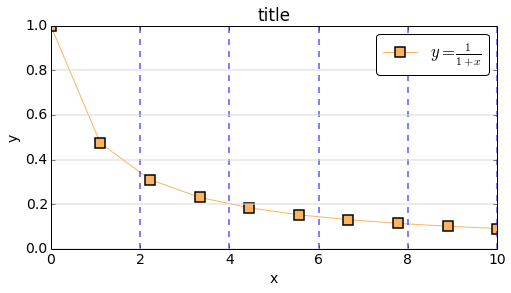
"""easyplot provides two ways to display the background grid for the axes.
- To display a simple grid without any custom formatting, the plot parameter
grid='on'can be passed to the easyplot object. Settinggrid='off'turns the grid off.
eplot.new_plot(x, 1/(1+x), '-s', label=r"$y = \frac{1}{1+x}$", c='#fdb462', grid='on')- For more advanced control of the grid, the easyplot
grid()instance method is provided with a call signature ofgrid(self, b=None, which='major', axis='both', **kwargs)where**kwargsare passed to linespec of grid lines (eg: linewidth=2)
    eplot.new_plot(x, 1/(1+x), '-s', label=r"$y = \frac{1}{1+x}$", c='#fdb462')
    eplot.grid(which='major', axis='x', linewidth=2, linestyle='--', color='b', alpha=0.5)
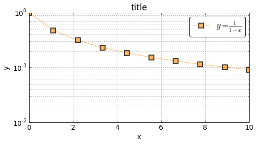
eplot.grid(which='major', axis='y', linewidth=2, linestyle='-', color='0.85', alpha=0.5)Plot parameters xscale and yscale can be passed to easyplot instances with
any of the following values: ['linear'|'log'|'symlog']
eplot.new_plot(x, 1/(1+x), '-s', label=r"$y = \frac{1}{1+x}$", c='#fdb462', yscale='log')
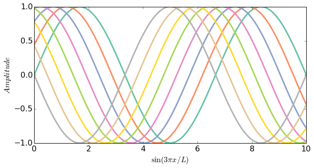
eplot.grid(which='minor', axis='both')easyplot provides the colorcycle plot parameter to specify the plot color
cycle. If the colorcycle parameter is passed with every add_plot command, it
will result in all plots using the first color of colorcycle. To avoid this,
the EasyPlot object should be initialized with the colorcycle and other plot
parameters without passing any x, y data as shown below. Subsequently, plots can
be added using the add_plot() method.
# Setup
colors = ["#66c2a5","#fc8d62","#8da0cb","#e78ac3","#a6d854","#ffd92f","#e5c494","#b3b3b3"]
x = np.linspace(0,10,200)

# Demo of color cycle
# Note the use of EasyPlot constructor with no x,y data to initialize colorcycle prior to
# adding plots to the figure
sinplot = EasyPlot(xlabel=r'$\sin (3\pi x/L)$', ylabel='$Amplitude$', fontsize=16, colorcycle=colors,
                   figsize=(10,5), linewidth=3)

for index in range(8):
sinplot.add_plot(x, np.sin(3*np.pi*x/10 + index*np.pi/7))The EasyPlot class has a very useful iter_plot() method to iterate through
x, y data stored in dictionaries or 2D arrays and plot them in a figure
using a single method call to iter_plot. The method signature of iter_plot
is as follows:
def iter_plot(self, x, y, mode='dict', **kwargs):
    """
    Plot multiple plots by iterating through x, y and parameter lists

    Arguments:
    ==========
      x : x values. 1D List/Array, Dictionary or Numpy 2D Array
      y : y values. Dictionary or 2D Python array (List of Lists where each
          sub-list is one set of y-data) or Numpy 2D Array
      mode : y, labels and other parameters should either be a Dictionary
             or a 2D Numpy array/2D List where each row corresponds to a
             single plot ['dict'|'array']
      **kwargs : Plot params as defined in __init__ documentation.
         Params can either be:
           scalars (same value applied to all plots),
           dictionaries (mode='dict', key[val] value applies to each plot)
           1D Lists/1D Numpy Arrays (mode='array', param[index] applies to each
           plot)
    """
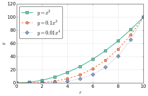
The examples below demonstrate the use of iter_plot to generate multiple plots
from a dataset using both mode settings, i.e., mode='dict' and
mode='array'. Note that single value plot parameters that are passed to
iter_plot (such as linewidth) are broadcast and applied to all plots in the
figure.
# Setup the x, y data and plot parameters for both modes
x = np.linspace(0, 10, 11)
dict_keys = ['x2', 'x3', 'x4']
labels_list = ['$y = x^2$', '$y = 0.1x^3$', '$y = 0.01x^4$']
markers_list = ['s', 'o', 'D']
linestyle_list = ['-', '--', ':']

y_dict, marker_dict, labels_dict, linestyle_dict = {}, {}, {}, {}
x_list, y_list = [], [] # List of x and y data sets for mode='array'

# Populate dict and list variables with data set
for ind, key in enumerate(dict_keys):
    marker_dict[key] = markers_list[ind]
    labels_dict[key] = labels_list[ind]
    linestyle_dict[key] = linestyle_list[ind]
    y_dict[key] = (0.1**ind)*x**(ind+2)
    y_list.append((0.1**ind)*x**(ind+2))
    x_list.append(x)


# Demonstrate iter_plot using mode='dict'
eplot = EasyPlot(xlabel=r'$x$', ylabel='$y$', fontsize=16,
                 colorcycle=["#66c2a5","#fc8d62","#8da0cb"], figsize=(8,5))
eplot.iter_plot(x, y_dict, linestyle=linestyle_dict, marker=marker_dict,
                label=labels_dict, linewidth=3, ms=10, showlegend=True, grid='on')
# Demonstrate iter_plot using mode='array'. Both x_list and y_list are 2D arrays
eplot = EasyPlot(xlabel=r'$x$', ylabel='$y$', fontsize=16,
colorcycle=["#66c2a5","#fc8d62","#8da0cb"], figsize=(8,5))
eplot.iter_plot(x_list, y_list, mode='array', linestyle=linestyle_list, marker=markers_list,
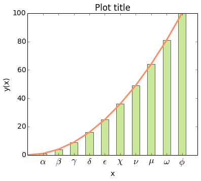
label=labels_list, linewidth=3, ms=10, showlegend=True, grid='on')EasyPlot objects provide access to their figure and axes objects via the
get_figure() and get_axes() methods. These methods can be used in
conjunction with regular object oriented matplotlib plotting methods (for
example the set and get methods on the axes object) to build more complex and
elaborate plots as shown in the examples below. The line_list instance
variable can also be accessed to obtain a list of [Line2D](http://matplotlib.o
rg/1.3.1/api/artist_api.html#matplotlib.lines.Line2D) items corresponding to the
plots in the figure. These can also then be manipulated using standard
matplotlib methods. When plotting interactively, the redraw() method must be
called on the easyplot object after any manipulation of the axes and figure
objects in order to update the plot display with the latest changes.
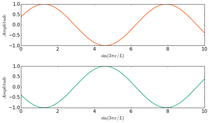
To create figures with subplots while taking advantage of an easyplot instance,
the axes and figure can be created by the user using pyplot.subplots,
gridspec or other common methods. The reference to the figure and and one of
the subplot axes can be passed to the easyplot instance method - new_plot() to
obtain the desired results as demonstrated below. The example below reuses the
sinplot object from this example as a template to easily
generate new plots with desired axis labels and plot parameters.
# Reuses sinplot template from one of the previous examples for labels, linewidth and fontsize
x = np.linspace(0, 10, 200)
fig, axes = plt.subplots(2, 1, figsize=(10,6)) # Create fig and axes for subplots externally

# Supply fig and axes instance to EasyPlot object
sinplot.new_plot(x, np.sin(3*np.pi*x/10 + np.pi/8), fig=fig, ax=axes[0], color="#fc8d62")
sinplot.new_plot(x, np.sin(3*np.pi*x/10 + 9*np.pi/8), fig=fig, ax=axes[1], color="#66c2a5")
fig.set_tight_layout(True)
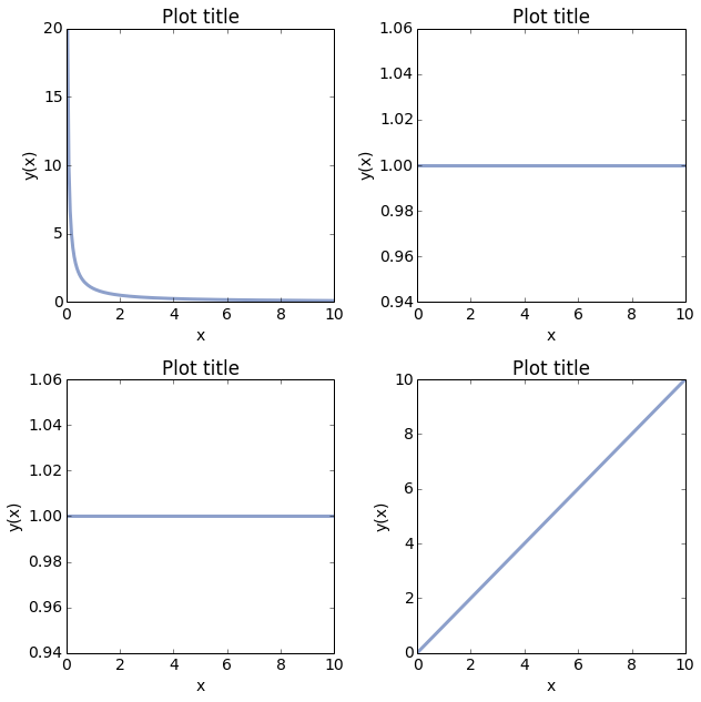
# Another example
fig, axes = plt.subplots(figsize=(9,9), nrows=2, ncols=2) # Create fig and axes
# Setup EasyPlot object with common plot parameters
eplot = EasyPlot(xlabel='x', ylabel='y(x)', title='Plot title', fs=14, lw=3)
# Loop through subplot axes and use eplot template to create new plots
for (x_ind,y_ind), ax in np.ndenumerate(axes):
eplot.new_plot(x, x**(x_ind+y_ind-1), fig=fig, ax=ax, c="#8da0cb")
fig.tight_layout()# Setup EasyPlot object with common plot parameters
x = np.linspace(0, 10, 11)
eplot = EasyPlot(x, x**2, xlabel='x', ylabel='y(x)', figsize=(6,5),
title='Plot title', fs=14, lw=3, xlim=(0,11), c="#fc8d62")
ax = eplot.get_axes()
# Modify plot by direct manipulation of axes instance
ax.bar(x, x**2, align="center", width=0.5, alpha=0.6, color="#a6d854")
ax.set_xticks([1, 2, 3, 4, 5, 6, 7, 8, 9, 10])
ax.set_xticklabels([r'$\alpha$', r'$\beta$', r'$\gamma$', r'$\delta$', r'$\epsilon$',
r'$\chi$', r'$\nu$', r'$\mu$', r'$\omega$', r'$\phi$'], fontsize=18)
eplot.redraw() # Update plot canvas with axes modifications