This repository is an accompaniment to an UNCTAD research paper (available here or here) benchmarking common nowcasting and machine learning methodologies. It illustrates how to estimate each of the methods examined in the analysis in either R or Python. 12 methodologies were tested in nowcasting quarterly US GDP using data from the Federal Reserve of Economic Data (FRED). The variables chosen were those specified in Bok, et al (2018). The methodologies were tested on three different test periods:
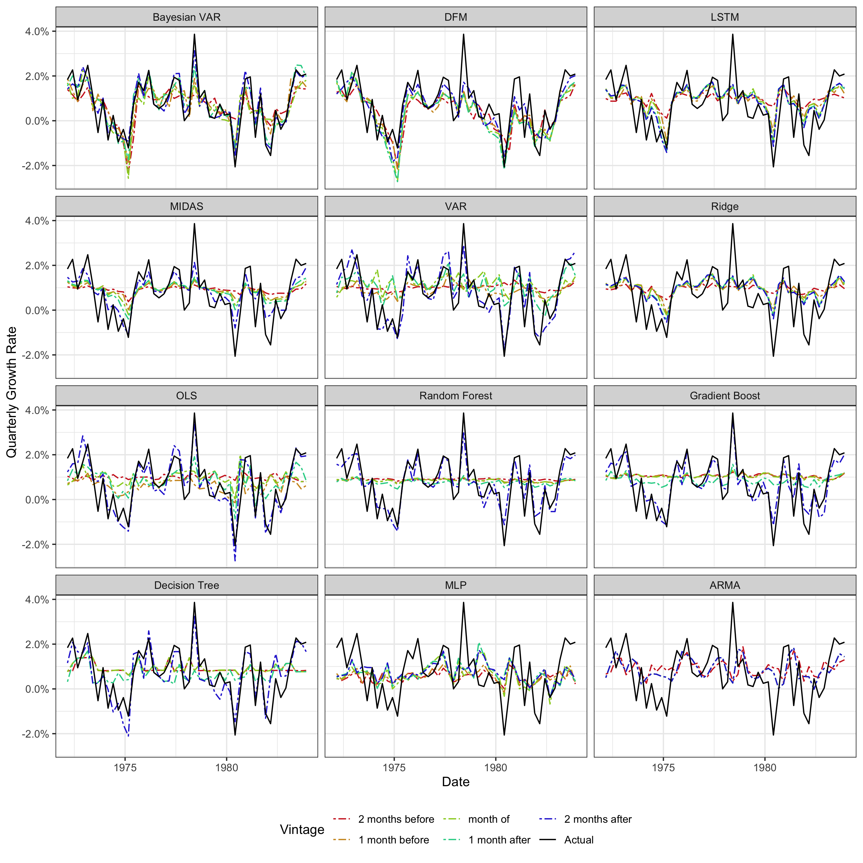
- the first quarter of 1972 to the fourth quarter of 1983 (test period 1, early 80s recession),
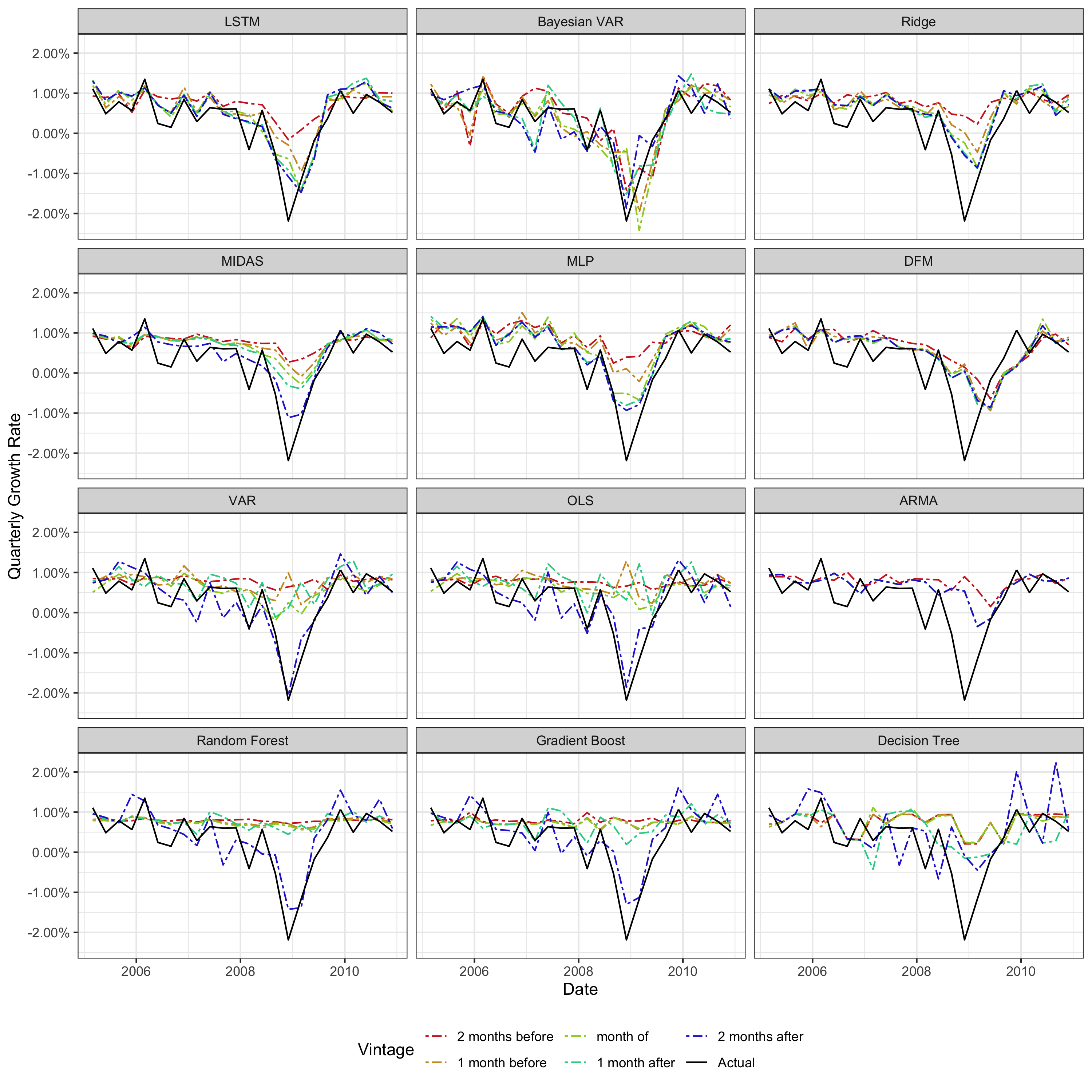
- the first quarter of 2005 to the fourth quarter of 2010 (test period 2, financial crisis),
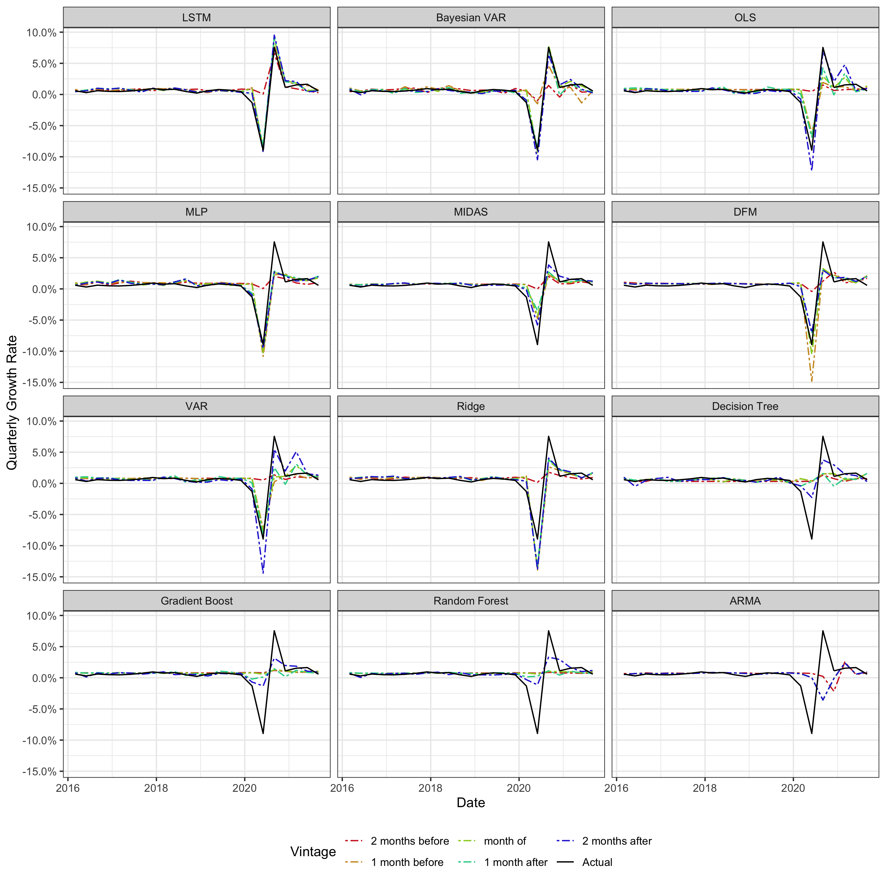
- the first quarter of 2016 to the third quarter of 2021 (test period 3, Covid crisis)
In applied nowcasting exercises, ideally, several methodologies should be employed and their results compared empirically for final model selection. In practice, this is difficult due to the fragmented landscape of different nowcasting methodology frameworks and implementations. This repository aims to make things significantly easier by giving fully runnable boilerplate code in R or Python for each methodology examined in this benchmarking analysis. The methodologies/ directory contains self-contained Jupyter notebooks illustrating how each methodology can be run in the nowcasting context with an example using a subset of data from FRED and testing on test period 2 (financial crisis). The results in these notebooks are meant as example and won't correspond exactly to the results in the paper (a smaller subset of variables is used for simplicity).
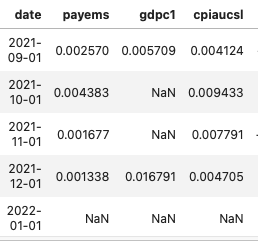
All the notebooks assume initial input data is in the format of seasonally adjusted growth rates in the highest frequency of the data (monthly in this case), with a date colum in the beginning and a separate column for each variable. Lower frequency data should have their values listed in the final month of that period (e.g. December for yearly data, March, June, September, or December for quarterly data), with no data / NAs in the intervening periods or for missing data at the end of series. An example is below.
Also necessary is a metadata CSV listing the name of the series/column and its frequency. Once these two conditions are met, it should be possible to run any of the methodologies on your own dataset, with adjustments as needed using the notebooks as a guide. Below is a short overview of each of the methodologies, followed by graphical results of the full benchmarking analysis showing predictions on different data vintages. The plots are ordered from best to worst performing in terms of RMSE for that test period.
If you only have bandwidth or interest to try out one methodology, the LSTM is recommended. It is accessible, available in four different programming languages, and straightforward to estimate and generate predictions given the data format stipulated above. It has shown strong predictive performance in relation to the other methodologies, including during shock conditions, and will not throw estimation errors on certain data. It does, however, have hyperparameters that may need to be tuned if initial performance is not good. This process can be done from within the nowcast_lstm library via the hyperparameter_tuning function. It is also the only implementation with built-in functionality for variable selection. In this analysis, input variables were taken as given, but often this is not the case. The variable_selection function will select best-performing variables from a pool of candidate variables. Both hyperparameter tuning and variable selection can also be performed together with the select_model function. See the documentation for the nowcast_lstm library for more information.
- ARMA (
model_arma.ipynb):- background: Wikipedia
- language, library, and function: Python,
ARIMAfunction ofpmdarimalibrary - commentary: Univariate benchmark model. Acceptable performance in normal/non-volatile times, extremely limited use during any shock periods. Potential use as another way to fill "ragged-edge" missing data for component series in other methodologies, as opposed to mean-filling.
- Bayesian mixed-frequency vector autoregression (
model_bvar.ipynb):- background: Wikipedia, ECB working paper
- language, library, and function: R,
estimate_mfbvarfunction ofmfbvarlibrary - commentary: Difficult to get data into proper format for the function to estimate properly, making dynamic/programmatic changing and selection of variables and overall usage hard, but doable. Very performant methodology in this benchmarking analysis, ranking the best in terms of RMSE for test period 1 (early 80s recession), and second-best in the second two periods (2008 financial crisis and Covid crisis) to the LSTM. However, predictions very volatile, with highest month-to-month revisions in predictions on average over all three test periods. Also may produce occasional large outlier predictions or fail to estimate on a dataset due to convergence, etc., issues. This library/implementation cannot handle yearly variables.
- Dynamic factor model (DFM) (
model_dfm.ipynb):- background: Wikipedia, FRB NY paper, UNCTAD research paper
- language, library, and function: R,
dfmfunction ofnowcastDFMlibrary - commentary: De facto standard in nowcasting, very commonly used. Usually good performance, second-best performance in first test period (early 80s financial crisis), but only sixth-best in second two test periods. May require assigning variables to different "blocks" or groups, which can be an added complication. In this benchmarking analysis, the DFM without blocks (equivalent to one "global" blocks/factor), performed very poorly in all but the first test period (early 80s recession). The model also fails to estimate on many datasets due to uninvertibility of matrices. Estimation may also take a long time depending on convergence of the expectation-maximization algorithm. Estimating models with more than 20 variables can be very slow. This library/implementation cannot handle yearly variables.
- Decision tree (
model_dt.ipynb):- background: Wikipedia
- language, library, and function: Python,
DecisionTreeRegressorfunction ofsklearnlibrary - commentary: Simple methodology, not traditionally used in nowcasting. Doesn't handle time series, handled via including additional variables for lags. Poor performance in this benchmarking analysis. The three tree-based methodologies in this analysis, decision trees, random forest, and gradient boost, learn most of their information from the latest available data, so have difficulties predicting things other than the mean in early data vintages. See
model_gb.ipynbfor a means of addressing this. All three also have difficulties predicting values more extreme than any they have seen before, limiting their use in shock periods, e.g. see third plot, Covid crisis. Has hyperparameters which may need to be tuned.
- Gradient boosted trees (
model_gb.ipynb):- background: Wikipedia
- language, library, and function: Python,
GradientBoostingRegressorfunction ofsklearnlibrary - commentary: Very performant model in traditional machine learning applications. Doesn't handle time series, handled via including additional variables for lags. Poor performance in this benchmarking analysis. However, performance can be substantially improved by training separate models for different data vintages, details in
model_gb.ipynbexample file. This method can be applied to any of the methodologies that don't handle time series (OLS, random forest, etc.), but it had the biggest positive impact in this benchmarking analysis for gradient boosted trees. Has hyperparameters which may need to be tuned.
- Long short-term memory neural network (LSTM) (
model_lstm.ipynb):- background: Wikipedia, first UNCTAD research paper, second UNCTAD research paper
- language, library, and function: Python,
LSTMfunction ofnowcast_lstmlibrary. Also available in Python, R, MATLAB, and Julia. - commentary: Very performant model, third-best performing model for first test period (early 80s recession), best-performing for second two (financial crisis and Covid crisis). Able to handle any frequency of data in either target or explanatory variables, easiest data setup process of any implementation in this benchmarking analysis. Couples high predictive performance with relatively low volatility, e.g. in contrast with Bayesian VAR, which also has good predictive performance, but is quite volatile. Can handle an arbitrarily large number of input variables without affecting estimation time and can be estimated on any dataset without error. Has hyperparameters which may need to be tuned.
- Mixed data sampling regression (MIDAS) (
model_midas.ipynb):- background: Wikipedia, paper
- language, library, and function: R,
midas_rfunction ofmidasrlibrary - commentary: Has been used in nowcasting, solid performance in this benchmarking analysis (fourth for the first two test periods, fifth for the third). Difficult data set up process to estimate and get predictions.
- Multilayer perceptron (feedforward) artificial neural network (
model_mlp.ipynb):- background: Wikipedia, paper
- language, library, and function: Python,
MLPRegressorfunction ofsklearnlibrary - commentary: Has been used in nowcasting, decent performance in this benchmarking analysis, except for the first test period (early 80s recession). Doesn't handle time series, handled via including additional variables for lags. Has hyperparameteres which may need to be tuned.
- Ordinary least squares regression (OLS) (
model_ols_ridge.ipynb):- background: Wikipedia
- language, library, and function: Python,
LinearRegressionfunction ofsklearnlibrary - commentary: Extremely popular approach to regression problems. Doesn't handle time series, handled via including additional variables for lags. Middling performance in this benchmarking analysis, will also probably suffer from multicollinearity if many variables are included.
- Ridge regression (
model_ols_ridge.ipynb):- background: Wikipedia
- language, library, and function: Python,
RidgeRegressionfunction ofsklearnlibrary - commentary: OLS with introduction of regularization penalty term. Can potentially help with multicollinearity issues of OLS in the nowcasting context. Performance is expectedly slightly better than that of OLS in this benchmarking analysis, with less volatile predictions. Introduces the ridge alpha hyperparameter which needs to be tuned.
- Random forest (
model_rf.ipynb):- background: Wikipedia
- language, library, and function: Python,
RandomForestRegressorfunction ofsklearnlibrary - commentary: Popular methodology in classical machine learning, combining the predictions of many random decision trees. Doesn't handle time series, handled via including additional variables for lags. Poor performance in this benchmarking analysis. Has hyperparameters which may need to be tuned.
- Mixed-frequency vector autoregression (VAR) (
model_var.ipynb):- background: Wikipedia, Minneapolis Fed paper
- language, library, and function: Python,
VARfunction ofPyFluxlibrary - commentary: Has been used in nowcasting. Middling performance in this benchmarking analysis. The PyFlux implementation can be difficult to get working and may not run on versions of Python > 3.5.


