SlicerBoneMorphing
Extension for 3D Slicer for bone mesh morphing.
At the moment, this module specializes for the humerus bone.
Special thanks <3
Special thanks goes to my wonderful colleagues Eva C. Herbst (@evaherbst) and Arthur Port (@agporto) for creating the initial idea and their huge help during the development of this module! Also, I would like to thank O. Hirose (@ohirose) for the research on BCPD/GBCPD and it's implementation (can be found here)
Installation
Supported platforms:
- Linux (x86_64)
- Windows (x86_64)
- MacOS (both x86_64 and ARM; Slicer runs through Rosetta on ARM-based Macs)
Steps:
- Download the latest ZIP package from Releases
- Extract the ZIP contents to your desired folder
- Open up 3D Slicer, go to Edit -> Application Settings
- In the modules section, add the extracted contents' path to "Additional Module Paths"
- Restart 3D Slicer
DISCLAIMER! After restarting, the installation process will begin. If there are any Python modules not available in Slicer, they will be installed, so the startup will take SIGNIFICANTLY MORE amount of time. Do not be scared, this is intended behaviour.
Usage
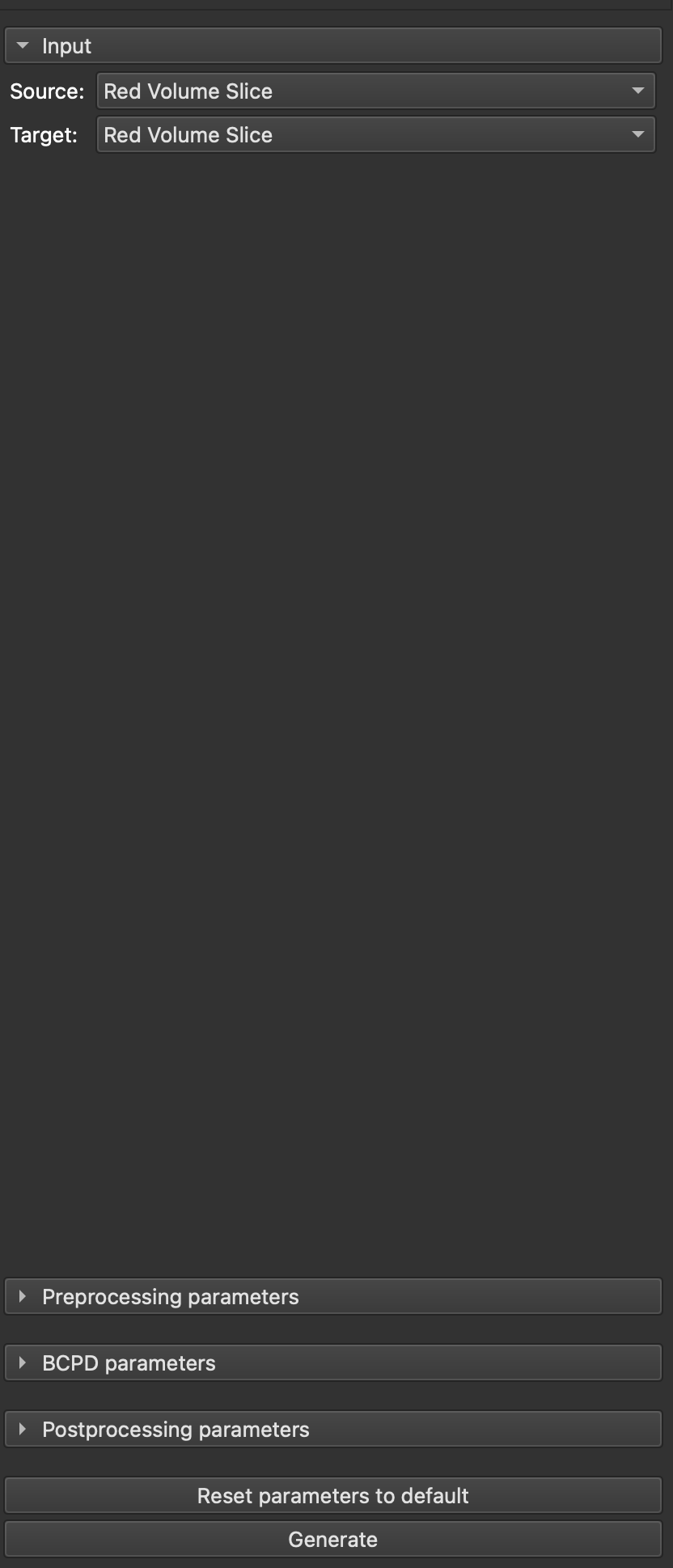
After a successful install, the module will be available in the Morphing section. When switching to the module, you should be greeted with the following UI:
The UI consists of 4 main sections
- Input
- Preprocessing
- Generation
- Postprocessing
Architecture
To be added.
Module sections
Input section
This section is self-explanatory. Here, you choose two input models:
- Source = Source for the generation; This is the model that represents the
- Target = Model which is non-complete => Needs its missing portions generated
Preprocessing section
Point cloud preprocessing
Before the generation process, we usually want to preprocess the model. Reasons could be to remove unwanted outliers or to smooth out the models. First of all, the model is converted to a point cloud to be able to effectively perform some preprocessing steps.
Then, a downsampling is performed. For this, you can configure the threshold for downsampling by the following parameter:
- Downsampling distance threshold
After the downsampling, we compute the normals of the point cloud. It uses a radius for which the normals are calculated and maximum number of neighbours. This can be adjusted with the following parameter:
- Normals estimation radius
- Normals estimation max neighbours
Also, we want calculate a Fast point feature histogram to somehow encode the local geometric properties. This method takes in two following parameters:
- FPFH search radius - Radius in which the FPFH is calculated in
- FPFH max neighbours - Maximum number of neighbours taken into account
Registration section
At this moment, we have our point clouds preprocessed and ready for the next step, which is the "registration" section. Here we try to define and calculate how and how much we need to adjust the source mesh to match the target one.
For this, we will use the downsampled point clouds with their corresponding FPFHs from the previous step. The concrete method we use is called RANSAC. It uses a process called "repeated random sub-sampling" to mitigate the effect of outliers and rotational differences as much as possible. The behaviour of this algorithm can be adjusted by the following parameters:
- Max iterations
- Distance threshold - same meaning as in previous steps
- Fitness threshold - the lowest fitness between the point clouds to be accepted. The lower, the higher chance of finding a good fit. The higher, higher the chance that either max iterations are reached
The result of the RANSAC algorithm is a bit "raw". To get the best possible fit, we perform the ICP registration algorithm upon the result. This can be tuned by the following parameter:
- ICP Distance threshold - same meaning as in previous steps
Generation section
Since we now have a preprocessed meshes and with defined transformations from the source to the target, we can proceed to the generation section.
For this purpose, we use a method called Bayesian coherent point drift. It falls into the non-rigid registration category of algorithms, which actually performs the deformation of the mesh to increase the fit of the source. It takes in both meshes and deforms the source into the target, similarly as we've already done in the Registration section. Due to the problem that BCPD allows for "unrealistic" deformations, we have done the pre-registration steps, which lets us mitigate the chance of getting into unrealistic deformations.
Now, BCPD allows for very fine adjustments of its behaviours using lots of different parameters. For the exact description of their effects, please refer to the documentation here.
Note: You do NOT have to perform any kind of installation process, the BCPD and its geodesic variant are already pre-built and preconfigured for immediate using in this module.
Not implemented options:
- Terminal output
- File output
Postprocessing section
After our models have been merged successfully, we still want to apply a slight amount of postprocessing to reach the most optimal results. We are basically using a bit of filtering and smoothing to the meshes. For these, we let you modify the following parameters:
- Clustering scaling - Scaled size of voxel for within vertices that are clustered together (additionally refer to here
- Smoothing iterations - Number of iterations of mesh smoothing
After the whole process is done, both the generated mesh (source transformed into target, standalone) and the merged mesh (generated meshes merged with the target; "combined model") are import back into the current Slicer scene.
FAQ
To be added.
Troubleshooting
To be added.

