Table Evaluator

Official documentation

TableEvaluator is a library to evaluate how similar a synthesized dataset is to a real data. In other words, it tries to give an indication into how real your fake data is. With the rise of GANs, specifically designed for tabular data, many applications are becoming possibilities. For industries like finance, healthcare and goverments, having the capacity to create high quality synthetic data that does not have the privacy constraints of normal data is extremely valuable. Since this field is this quite young and developing, I created this library to have a consistent evaluation method for your models.

Installation

The package can be installed with

pip install table_evaluator

Tests

The test can be run by cloning the repo and running:

pytest tests

Usage

Please see the example notebook for the most up-to-date examples. The README example is just that notebook, but sometimes a bit outdated. Start by importing the class

from table_evaluator import load_data, TableEvaluator

The package is used by having two DataFrames; one with the real data and one with the synthetic data. These are passed to the TableEvaluator on init. The utils.load_data is nice to retrieve these dataframes from disk since it converts them to the same dtypes and columns after loading. However, any dataframe will do as long as they have the same columns and data types.

Using the test data available in the data directory, we do:

real, fake = load_data('data/real_test_sample.csv', 'data/fake_test_sample.csv')

which gives us two dataframes and specifies which columns should be treated as categorical columns.

real.head()

trans_id	account_id	trans_amount	balance_after_trans	trans_type	trans_operation	trans_k_symbol	trans_date
951892	3245	3878.0	13680.0	WITHDRAWAL	REMITTANCE_TO_OTHER_BANK	HOUSEHOLD	2165
3547680	515	65.9	14898.6	CREDIT	UNKNOWN	INTEREST_CREDITED	2006
1187131	4066	32245.0	57995.5	CREDIT	COLLECTION_FROM_OTHER_BANK	UNKNOWN	2139
531421	1811	3990.8	23324.9	WITHDRAWAL	REMITTANCE_TO_OTHER_BANK	LOAN_PAYMENT	892
37081	119	12100.0	36580.0	WITHDRAWAL	WITHDRAWAL_IN_CASH	UNKNOWN	654

fake.head()

trans_id	account_id	trans_amount	balance_after_trans	trans_type	trans_operation	trans_k_symbol	trans_date
911598	3001	13619.0	92079.0	CREDIT	COLLECTION_FROM_OTHER_BANK	UNKNOWN	1885
377371	1042	4174.0	32470.0	WITHDRAWAL	REMITTANCE_TO_OTHER_BANK	HOUSEHOLD	1483
970113	3225	274.0	57608.0	WITHDRAWAL	WITHDRAWAL_IN_CASH	UNKNOWN	1855
450090	1489	301.0	36258.0	CREDIT	CREDIT_IN_CASH	UNKNOWN	885
1120409	3634	6303.0	50975.0	WITHDRAWAL	REMITTANCE_TO_OTHER_BANK	HOUSEHOLD	1211

cat_cols = ['trans_type', 'trans_operation', 'trans_k_symbol']

If we do not specify categorical columns when initializing the TableEvaluator, it will consider all columns with more than 50 unique values a continuous column and anything with less a categorical columns.

Then we create the TableEvaluator object:

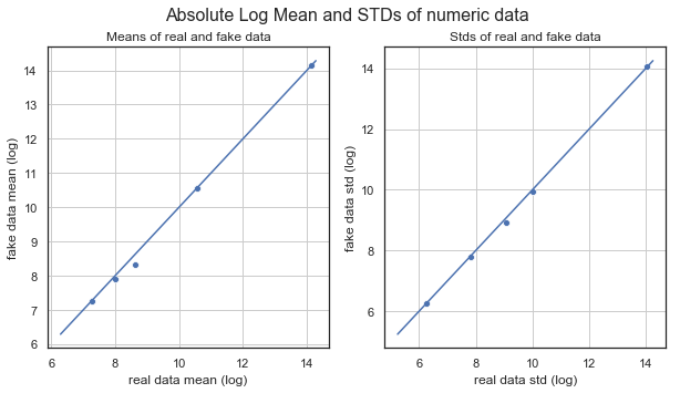
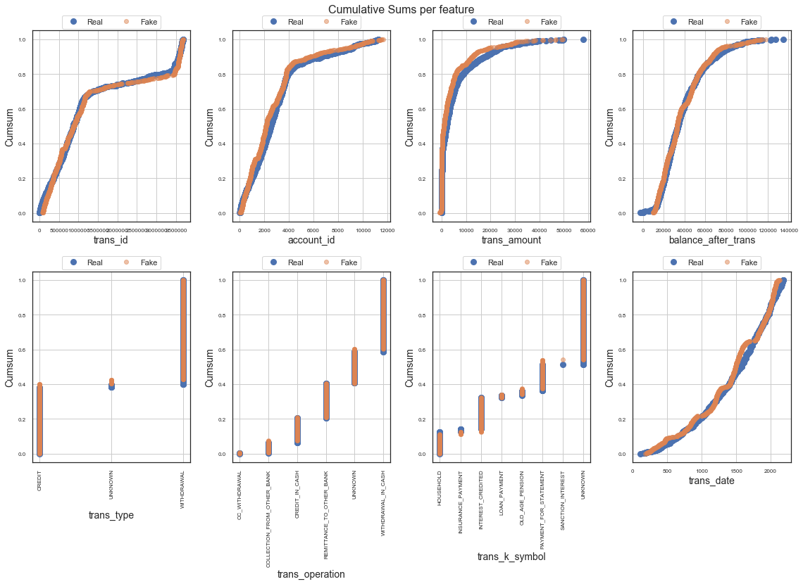
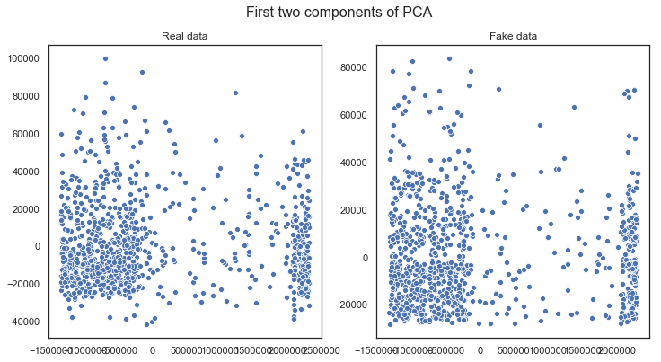
table_evaluator = TableEvaluator(real, fake, cat_cols=cat_cols)

It's nice to start with some plots to get a feel for the data and how they correlate. The test samples contain only 1000 samples, which is why the cumulative sum plots are not very smooth.

table_evaluator.visual_evaluation()

The evaluate method gives us the most complete idea of how close the data sets are together.

table_evaluator.evaluate(target_col='trans_type')

Correlation metric: pearsonr

Classifier F1-scores:
                                      real   fake
real_data_LogisticRegression_F1     0.8200 0.8150
real_data_RandomForestClassifier_F1 0.9800 0.9800
real_data_DecisionTreeClassifier_F1 0.9600 0.9700
real_data_MLPClassifier_F1          0.3500 0.6850
fake_data_LogisticRegression_F1     0.7800 0.7650
fake_data_RandomForestClassifier_F1 0.9300 0.9300
fake_data_DecisionTreeClassifier_F1 0.9300 0.9400
fake_data_MLPClassifier_F1          0.3600 0.6200

Miscellaneous results:
                                  Result
Column Correlation Distance RMSE          0.0399
Column Correlation distance MAE           0.0296
Duplicate rows between sets (real/fake)   (0, 0)
nearest neighbor mean                     0.5655
nearest neighbor std                      0.3726

Results:
                                                Result
basic statistics                                0.9940
Correlation column correlations                 0.9904
Mean Correlation between fake and real columns  0.9566
1 - MAPE Estimator results                      0.7843
1 - MAPE 5 PCA components                       0.9138
Similarity Score                                0.9278

The similarity score is an aggregate metric of the five other metrics in the section with results. Additionally, the F1/RMSE scores are printed since they give valuable insights into the strengths and weaknesses of some of these models. Lastly, some miscellaneous results are printed, like the nearest neighbor distance between each row in the fake dataset and the closest row in the real dataset. This provides insight into the privacy retention capability of the model. Note that the mean and standard deviation of nearest neighbor is limited to 20k rows, due to time and hardware limitations.

Full Documentation

Please see the full documentation on https://baukebrenninkmeijer.github.io/table-evaluator/.

Motivation

To see the motivation for my decisions, please have a look at my master thesis, found at https://www.ru.nl/publish/pages/769526/z04_master_thesis_brenninkmeijer.pdf

If you have any tips or suggestions, please contact send me on email.