Fast sf-to-raster conversion
fasterize is a high-performance replacement for the rasterize() function in the raster package.
Functionality is currently limited to rasterizing polygons in sf-type data frames.
Install the current version of fasterize from CRAN:
install.packages('fasterize')Install the development version of fasterize with devtools:
devtools::install_github("ecohealthalliance/fasterize")fasterize uses Rcpp and thus requires a compile toolchain to install from source. Testing (and most use) requires sf, which requires GDAL (>= 2.0.0), GEOS (>= 3.3.0), and PROJ.4 (>= 4.8.0) to be installed on your system.
The main function, fasterize(), takes the same inputs as raster::rasterize() but currently has fewer options and is is limited to rasterizing polygons.
A method for creating empty rasters from sf objects is provided, and raster plot methods are re-exported.
library(raster)
library(fasterize)
library(sf)
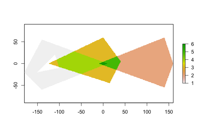
p1 <- rbind(c(-180,-20), c(-140,55), c(10, 0), c(-140,-60), c(-180,-20))
hole <- rbind(c(-150,-20), c(-100,-10), c(-110,20), c(-150,-20))
p1 <- list(p1, hole)
p2 <- list(rbind(c(-10,0), c(140,60), c(160,0), c(140,-55), c(-10,0)))
p3 <- list(rbind(c(-125,0), c(0,60), c(40,5), c(15,-45), c(-125,0)))
pols <- st_sf(value = c(1,2,3),
             geometry = st_sfc(lapply(list(p1, p2, p3), st_polygon)))
r <- raster(pols, res = 1)
r <- fasterize(pols, r, field = "value", fun="sum")
plot(r)Let's compare fasterize() to raster::rasterize():
pols_r <- as(pols, "Spatial")
bench <- microbenchmark::microbenchmark(
  rasterize = r <- raster::rasterize(pols_r, r, field = "value", fun="sum"),
  fasterize = f <- fasterize(pols, r, field = "value", fun="sum"),
  unit = "ms"
)
print(bench, digits = 3)
#> Unit: milliseconds
#> expr min lq mean median uq max neval cld
#> rasterize 342.486 379.028 426.959 404.759 434.029 859.01 100 b
#> fasterize 0.337 0.368 0.499 0.413 0.636 2.02 100 a
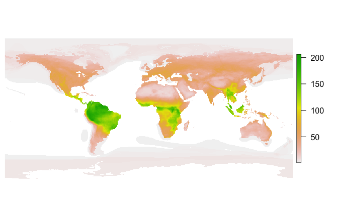
How does fasterize() do on a large set of polygons? Here I download the IUCN shapefile for the ranges of all terrestrial mammals and generate a 1/6 degree world map of mammalian biodiversity by rasterizing all the layers.
if(!dir.exists("Mammals_Terrestrial")) {
  download.file(
    "https://s3.amazonaws.com/hp3-shapefiles/Mammals_Terrestrial.zip",
    destfile = "Mammals_Terrestrial.zip") # <-- 383 MB
  unzip("Mammals_Terrestrial.zip", exdir = ".")
  unlink("Mammals_Terrestrial.zip")
}
mammal_shapes <- st_read("Mammals_Terrestrial")#> Reading layer `Mammals_Terrestrial' from data source `/Users/noamross/dropbox-eha/projects-eha/fasterize/Mammals_Terrestrial' using driver `ESRI Shapefile'
#> Simple feature collection with 42714 features and 27 fields
#> geometry type: MULTIPOLYGON
#> dimension: XY
#> bbox: xmin: -180 ymin: -85.58276 xmax: 180 ymax: 89.99999
#> epsg (SRID): 4326
#> proj4string: +proj=longlat +datum=WGS84 +no_defs
mammal_raster <- raster(mammal_shapes, res = 1/6)
bench2 <- microbenchmark::microbenchmark(
  mammals = mammal_raster <- fasterize(mammal_shapes, mammal_raster, fun="sum"),
  times=20, unit = "s")
print(bench2, digits=3)
#> Unit: seconds
#> expr min lq mean median uq max neval
#> mammals 0.847 0.857 0.883 0.886 0.894 0.963 20
par(mar=c(0,0.5,0,0.5))
plot(mammal_raster, axes=FALSE, box=FALSE)fasterize is developed openly at EcoHealth Alliance under the USAID PREDICT project. Please note that this project is released with a Contributor Code of Conduct. By participating in this project you agree to abide by its terms.


