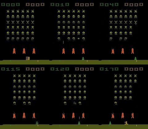
Notebook utilizing Deep Q-learning and Epsilon Greedy Policies to tackle the OpenAI Space Invaders environment, where we explore the importance of Data Preprocessing through frame composition and stacking.
- Frame stacking: the joining of several game frames together to provide a temporal reference of our game environment.
- Frame composition: the element-wise maximization of two game frames together to provide a motion reference that also overcomes the issue of partial rendering.
An article for TowardsDataScience.
- We define our Deep Q-learning neural network. This is a CNN that takes in-game screen images and outputs the probabilities of each of the actions, or Q-values, in the Ms-Pacman gamespace. To acquire a tensor of probabilitieses, we do not include any activation function in our final layer.
- As Q-learning require us to have knowledge of both the current and next states, we need to start with data generation. We feed preprocessed input images of the game space, representing initial states s, into the network, and acquire the initial probability distribution of actions, or Q-values. Before training, these values will appear random and sub-optimal. Note that our preprocessing now includes stacking and composition as well.
- With our tensor of probabilities, we then select the action with the current highest probability using the argmax() function, and use it to build an epsilon greedy policy.
- Using our policy, we'll then select the action a, and evaluate our decision in the gym environment to receive information on the new state s', the reward r, and whether the episode has been finished.
- We store this combination of information in a buffer in the list form <s,a,r,s',d>, and repeat steps 2–4 for a preset number of times to build up a large enough buffer dataset.
- Once step 5 has finished,we move to generate our target y-values, R' and A', that are required for the loss calculation. While the former is simply discounted from R, we obtain the A' by feeding S' into our network. With all of our components in place, we can then calculate the loss to train our network.
- Once training has finished, we'll evaluate the performance of our agent graphically and through a demonstration
