The R package BGGM provides tools for making Bayesian inference in
Gaussian graphical models (GGM). The methods are organized around two
general approaches for Bayesian inference: (1) estimation and (2)
hypothesis testing. The key distinction is that the former focuses on
either the posterior or posterior predictive distribution (Gelman, Meng,
and Stern 1996; see section 5 in Rubin 1984), whereas the latter focuses
on model comparison with the Bayes factor (Jeffreys 1961; Kass and
Raftery 1995).
A Gaussian graphical model captures conditional (in)dependencies among a set of variables. These are pairwise relations (partial correlations) controlling for the effects of all other variables in the model.
The Gaussian graphical model is used across the sciences, including (but not limited to) economics (Millington and Niranjan 2020), climate science (Zerenner et al. 2014), genetics (Chu et al. 2009), and psychology (Rodriguez et al. 2020).
To install the latest release version (2.0.0) from CRAN use
install.packages("BGGM") The current developmental version can be installed with
if (!requireNamespace("remotes")) {
  install.packages("remotes")
}
remotes::install_github("donaldRwilliams/BGGM")The methods in BGGM build upon existing algorithms that are well-known in the literature. The central contribution of BGGM is to extend those approaches:
-
Bayesian estimation with the novel matrix-F prior distribution (Mulder and Pericchi 2018)
- Estimation (Williams 2018)
-
Bayesian hypothesis testing with the matrix-F prior distribution (Williams and Mulder 2019)
-
Comparing Gaussian graphical models (Williams 2018; Williams et al. 2020)
-
Extending inference beyond the conditional (in)dependence structure (Williams 2018)
-
Posterior uncertainty intervals for the partial correlations
The computationally intensive tasks are written in c++ via the R
package Rcpp (Eddelbuettel et al. 2011) and the c++ library
Armadillo (Sanderson and Curtin 2016). The Bayes factors are
computed with the R package BFpack (Mulder et al. 2019).
Furthermore, there are plotting functions for
each method, control variables can be included in the model (e.g., ~ gender), and there is support for missing values (see bggm_missing).
-
Continuous: The continuous method was described in Williams (2018). Note that this is based on the customary Wishart distribution.
-
Binary: The binary method builds directly upon Talhouk, Doucet, and Murphy (2012) that, in turn, built upon the approaches of Lawrence et al. (2008) and Webb and Forster (2008) (to name a few).
-
Ordinal: The ordinal methods require sampling thresholds. There are two approach included in BGGM. The customary approach described in Albert and Chib (1993) (the default) and the ‘Cowles’ algorithm described in Cowles (1996).
-
Mixed: The mixed data (a combination of discrete and continuous) method was introduced in Hoff (2007). This is a semi-parametric copula model (i.e., a copula GGM) based on the ranked likelihood. Note that this can be used for only ordinal data (not restricted to “mixed” data).
The following includes brief examples for some of the methods in BGGM.
An ordinal GGM is estimated with
library(BGGM)
library(ggplot2)

# data
Y <- ptsd[,1:5] + 1

# ordinal
fit <- estimate(Y, type = "ordinal",
                analytic = FALSE)
Notice the + 1. This is required, because the first category must be
1 when type = "ordinal". The partial correlations can the be
summarized with
summary(fit)

#> BGGM: Bayesian Gaussian Graphical Models
#> ---
#> Type: ordinal
#> Analytic: FALSE
#> Formula:
#> Posterior Samples: 250
#> Observations (n):
#> Nodes (p): 5
#> Relations: 10
#> ---
#> Call:
#> estimate(Y = Y, type = "ordinal", analytic = FALSE, iter = 250)
#> ---
#> Estimates:
#>  Relation Post.mean Post.sd Cred.lb Cred.ub
#>    B1--B2     0.258   0.079   0.105   0.418
#>    B1--B3     0.028   0.086  -0.127   0.189
#>    B2--B3     0.517   0.058   0.406   0.616
#>    B1--B4     0.356   0.070   0.210   0.486
#>    B2--B4    -0.076   0.078  -0.219   0.063
#>    B3--B4     0.246   0.077   0.107   0.385
#>    B1--B5     0.131   0.080  -0.020   0.279
#>    B2--B5     0.127   0.083  -0.040   0.284
#>    B3--B5     0.202   0.079   0.063   0.366
#>    B4--B5     0.349   0.070   0.209   0.474
#> ---
The returned object can also be plotted, which allows for visualizing the posterior uncertainty interval for each relation. An example is provided below in Posterior uncertainty intervals. The partial correlation matrix is accessed with
pcor_mat(fit)| B1 | B2 | B3 | B4 | B5 | |
|---|---|---|---|---|---|
| B1 | 0.000 | 0.258 | 0.028 | 0.356 | 0.131 |
| B2 | 0.258 | 0.000 | 0.517 | -0.076 | 0.127 |
| B3 | 0.028 | 0.517 | 0.000 | 0.246 | 0.202 |
| B4 | 0.356 | -0.076 | 0.246 | 0.000 | 0.349 |
| B5 | 0.131 | 0.127 | 0.202 | 0.349 | 0.000 |
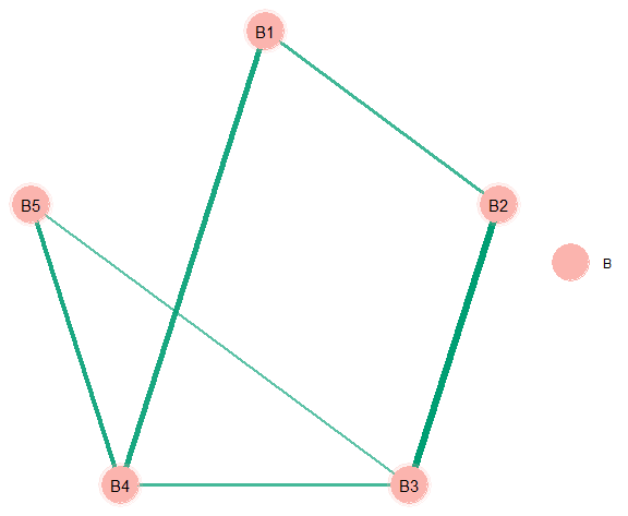
The graph is selected with
E <- select(fit)and then plotted
# "communities"
comm <- substring(colnames(Y), 1, 1)

plot(select(fit),
     groups = comm,
     edge_magnify = 5,
     palette = "Pastel1",
     node_size = 12)
This basic “workflow” can be used with all methods and data types. A more involved network plot is provided below.
There is also an analytic solution that is based on the Wishart
distribution. This simple solution provides competitive performance with
“state-of-the-art” methods, assuming that n (observations) > p
(variables). The one caveat is that it works only for type = "continuous" (the default).
# analytic
fit <- estimate(Y, analytic = TRUE)

# network plot
plot(select(fit))
This is quite handy when (1) only the conditional dependence structure is of interest and (2) an immediate solution is desirable. An example of (2) is provided in Posterior Predictive Check.
The Bayes factor based methods allow for determining the conditional independence structure (evidence for the null hypothesis).
# now 10 nodes
Y <- ptsd[,1:10]

# exploratory hypothesis testing
fit<- explore(Y)

# select
E <- select(fit, alternative = "exhaustive")
The option alternative = "exhaustive" compares three hypotheses: (1) a
null relation; (2) a positive relation; and (3) a negative relation.
summary(E)

#> BGGM: Bayesian Gaussian Graphical Models
#> ---
#> Type: ordinal
#> Alternative: exhaustive
#> ---
#> Call:
#> select.explore(object = fit, alternative = "exhaustive")
#> ---
#> Hypotheses:
#> H0: rho = 0
#> H1: rho > 0
#> H2: rho < 0
#> ---
#>
#>  Relation Post.mean Post.sd Pr.H0 Pr.H1 Pr.H2
#>  B1--B2    0.263    0.080   0.000 0.999 0.001
#>  B1--B3    0.020    0.081   0.710 0.173 0.116
#>  B2--B3    0.523    0.073   0.000 1.000 0.000
#>  B1--B4    0.362    0.070   0.000 1.000 0.000
#>  B2--B4   -0.082    0.068   0.459 0.061 0.480
#>  B3--B4    0.252    0.073   0.000 1.000 0.000
#>  B1--B5    0.129    0.072   0.120 0.847 0.033
#>  B2--B5    0.118    0.078   0.223 0.726 0.051
#>  B3--B5    0.213    0.077   0.001 0.996 0.003
#>  B4--B5    0.348    0.072   0.000 1.000 0.000
The posterior hypothesis probabilities are provided in the last three
columns. When using plot(E), there is a network plot for each
hypothesis.
A central contribution of BGGM is confirmatory hypothesis testing of
(in)equality constraints (Hoijtink 2011). By this we are referring to
testing expectations, as opposed to feeding the data to, say,
estimate, and seeing what happens to emerge.
In this example, the focus is on suicidal thoughts (PHQ9) in a
comorbidity network. Here is an example set of hypotheses
# data (+ 1)
Y <- depression_anxiety_t1 + 1

# example hypotheses
hyp <- c("PHQ2--PHQ9 > PHQ1--PHQ9 > 0;
          PHQ2--PHQ9 = PHQ1--PHQ9 = 0")
There are two hypotheses separated by (;). The first expresses that
the relation PHQ2--PHQ9 (“feeling down, depressed, or hopeless” and
“suicidal thoughts”) is larger than PHQ1--PHQ9 (“little interest or
pleasure in doing things” and “suicidal thoughts”). In other words, that
the partial correlation is larger for PHQ2--PHQ9. There is an
additional constraint to positive values (> 0) for both relations. The
second hypothesis is then a “null” model.
# (try to) confirm
fit <- confirm(Y = Y, hypothesis = hyp,
               type = "ordinal")
The object fit is then printed
fit

#> BGGM: Bayesian Gaussian Graphical Models
#> Type: ordinal
#> ---
#> Posterior Samples: 250
#> Observations (n): 403
#> Variables (p): 16
#> Delta: 15
#> ---
#> Call:
#> confirm(Y = Y + 1, hypothesis = hyp, type = "ordinal",
#>     iter = 250)
#> ---
#> Hypotheses:
#>
#> H1: PHQ2--PHQ9>PHQ1--PHQ9>0
#> H2: PHQ2--PHQ9=PHQ1--PHQ9=0
#> H3: complement
#> ---
#> Posterior prob:
#>
#> p(H1|data) = 0.895
#> p(H2|data) = 0.002
#> p(H3|data) = 0.103
#> ---
#> Bayes factor matrix:
#>       H1      H2    H3
#> H1 1.000 529.910 8.666
#> H2 0.002   1.000 0.016
#> H3 0.115  61.147 1.000
#> ---
#> note: equal hypothesis prior probabilities
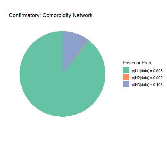
The posterior hypothesis probability is 0.895 which provides some
evidence for the order constraint. The Bayes factor matrix then divides
the posterior probabilities. This provide a measure of relative
support for which hypothesis the data were more likely under.
Finally, the results can be plotted
plot(fit) +
  scale_fill_brewer(palette = "Set2",
                    name = "Posterior Prob") +
  ggtitle("Confirmatory: Comorbidity Network")
This demonstrates that all the plot() functions in BGGM return
ggplot objects that can be further customized. Note that BGGM is
not focused on making publication ready plots. Typically the bare
minimum is provided that can then be honed in.
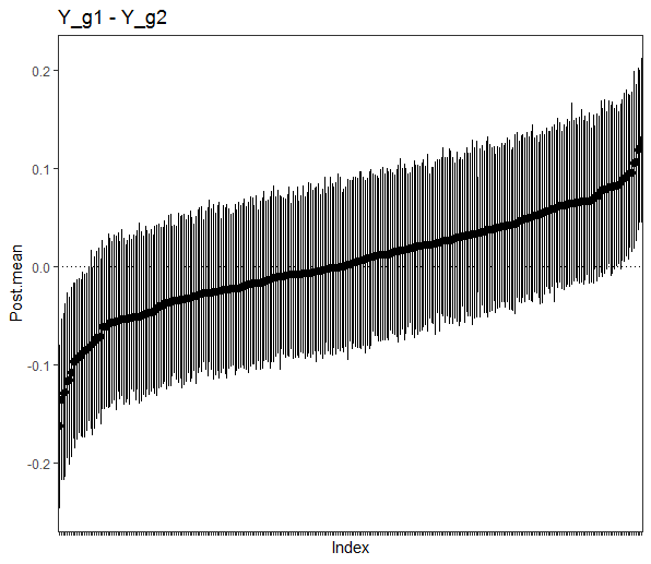
This method compares groups by computing the difference for each relation in the model. In other words, there are pairwise contrasts for each partial correlation, resulting in a posterior distribution for each difference.
In all examples in this section, personality networks are compared for males and females.
# data
Y <- bfi

# males
Ymales <- subset(Y, gender == 1,
                 select = -c(gender, education))

# females
Yfemales <- subset(Y, gender == 2,
                 select = -c(gender, education))
Fit the model
fit <- ggm_compare_estimate(Ymales, Yfemales)Then plot the results, in this case the posterior distribution for each difference
# plot summary
plot(summary(fit))
Note that it is also possible to use select for the object fit and
then plot the results. This produces a network plot including the
selected differences. Furthermore, it is also possible to plot the
partial correlations (not the differences). This is accomplished by
using plot with the summary computed from an estimate object (see
above).
The predictive check method uses Jensen-Shannon divergence (i.e., symmetric Kullback-Leibler divergence Wikipedia) and the sum of squared error (for the partial correlation matrices) to compare groups (Williams et al. 2020).
The following compares the groups
fit <- ggm_compare_ppc(Ymales, Yfemales)Then print the summary output with
fit

#> BGGM: Bayesian Gaussian Graphical Models
#> ---
#> Test: Global Predictive Check
#> Posterior Samples: 500
#>   Group 1: 805
#>   Group 2: 1631
#> Nodes:  25
#> Relations: 300
#> ---
#> Call:
#> ggm_compare_ppc(Ymales, Yfemales, iter = 500)
#> ---
#> Symmetric KL divergence (JSD):
#>
#>    contrast JSD.obs p_value
#>  Yg1 vs Yg2   0.442       0
#> ---
#>
#> Sum of Squared Error:
#>
#>    contrast SSE.obs p.value
#>  Yg1 vs Yg2   0.759       0
#> ---
#> note:
#> JSD is Jensen-Shannon divergence
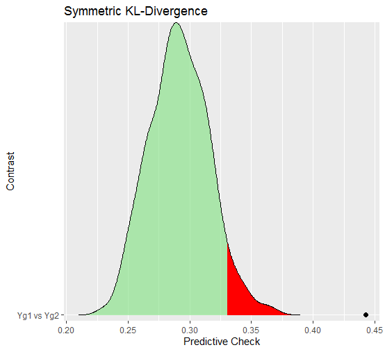
In this case, there seems to be decisive evidence that the networks are different (as indicated by the posterior predictive p-value). The predictive distribution can also be plotted
plot(fit,
     critical = 0.05)$plot_jsd
where the red region is the “critical” area and the black point is the observed KL divergence for the networks. This again shows that the “distance” between the networks is much more than expected, assuming that the groups were actually the same.
This next example is a new feature in BGGM (2.0.0), that allows
for comparing GGMs any way the user wants. All that is required is to
(1) decide on a test-statistic and (2) write a custom function.
Here is an example using Hamming distance (Wikipedia), which is essentially the squared error between adjacency matrices (a test for different structures).
First define the custom function
f <- function(Yg1, Yg2){

# remove NA
x <- na.omit(Yg1)
y <- na.omit(Yg2)

# nodes
p <- ncol(x)

# identity matrix
I_p <- diag(p)

# estimate graphs
fit1 <-  estimate(x, analytic = TRUE)
fit2 <-  estimate(y, analytic = TRUE)

# select graphs
sel1 <- select(fit1)
sel2 <- select(fit2)

# Hamming distance
sum((sel1$adj[upper.tri(I_p)] - sel2$adj[upper.tri(I_p)])^2)
}
Note that (1) analytic = TRUE is being used, which is needed in this
case because two graphs are estimated for each iteration (or draw from
the posterior predictive distribution) and (2) f requires two datasets
as the input and returns a single number (the chosen test-statistic).
The next step is to compute the observed Hamming distance
# observed difference
obs <- f(Ymales, Yfemales)
then compare the groups
fit <- ggm_compare_ppc(Ymales, Yfemales,
                             FUN = f,
                             custom_obs  = obs)

# print
fit

#> BGGM: Bayesian Gaussian Graphical Models
#> ---
#> Test: Global Predictive Check
#> Posterior Samples: 250
#>   Group 1: 805
#>   Group 2: 1631
#> Nodes:  25
#> Relations: 300
#> ---
#> Call:
#> ggm_compare_ppc(Ymales, Yfemales, iter = 250, FUN = f, custom_obs = obs)
#> ---
#> Custom:
#>
#>    contrast custom.obs p.value
#>  Yg1 vs Yg2         75   0.576
#> ---
In this case, the p-value does not indicate that the groups are different for this test-statistic. This may seem contradictory to the previous results, but it is important to note that Hamming distance asks a much different question related to the adjacency matrices (no other information, such as edge weights, is considered).
The Bayes factor based methods allow for determining the conditional independence structure (evidence for the null hypothesis), in this case for group equality.
Fit the model
fit <- ggm_compare_explore(Ymales, Yfemales)Then plot the results
plot(summary(fit)) +
  theme_bw() +
  theme(panel.grid = element_blank(),
        axis.text.y = element_blank())
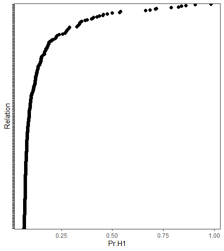
Here the posterior probability for a difference is visualized for each
relation in the GGM. Note that it is also possible to use select for
the object fit and then plot the results. This produces a network plot
including the selected differences, in addition to a plot depicting the
relations for which there was evidence for the null hypothesis.
A central contribution of BGGM is confirmatory hypothesis testing of
(in)equality constraints (Hoijtink 2011), in this case for comparing
groups. By this we are referring to testing expectations, as opposed to
feeding the data to, say, estimate, and seeing what happens to emerge.
In this example, the focus is on agreeableness in a personality network. Here is a set of hypotheses
hyp <- c("g1_A2--A4 > g2_A2--A4 > 0 & g1_A4--A5 > g2_A4--A5 > 0;
          g1_A4--A5 = g2_A4--A5 = 0  & g1_A2--A4 = g2_A2--A4 = 0")
where the variables are A2 (“inquire about others’ well being”), A4
(“love children”), and A5 (“make people feel at ease”). The first
hypothesis states that the conditionally dependent effects are larger
for female than males (note the &), with the additional constraint to
positive values, whereas the second hypothesis is a “null” model.
The hypothesis is tested with the following
fit <- ggm_compare_confirm(Yfemales, Ymales,
                           hypothesis = hyp)

# print
fit

#> BGGM: Bayesian Gaussian Graphical Models
#> Type: continuous
#> ---
#> Posterior Samples: 500
#>   Group 1: 1631
#>   Group 2: 805
#> Variables (p): 25
#> Relations: 300
#> Delta: 15
#> ---
#> Call:
#> ggm_compare_confirm(Yfemales, Ymales, hypothesis = hyp, iter = 500)
#> ---
#> Hypotheses:
#>
#> H1: g1_A2--A4>g2_A2--A4>0&g1_A4--A5>g2_A4--A5>0
#> H2: g1_A4--A5=g2_A4--A5=0&g1_A2--A4=g2_A2--A4=0
#> H3: complement
#> ---
#> Posterior prob:
#>
#> p(H1|data) = 0.989
#> p(H2|data) = 0
#> p(H3|data) = 0.011
#> ---
#> Bayes factor matrix:
#>       H1           H2     H3
#> H1 1.000 1.180798e+14 92.115
#> H2 0.000 1.000000e+00  0.000
#> H3 0.011 1.281873e+12  1.000
#> ---
#> note: equal hypothesis prior probabilities
The posterior hypothesis probability is 0.989 which provides strong evidence for the hypothesis that predicted these “agreeableness” relations would be larger in females than in males. This can also be plotted, as in Confirmatory (one group). See Rodriguez et al. (2020) for a full treatment of confirmatory testing in substantive applications.
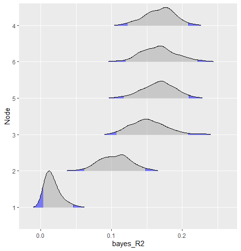
In this example, predictability is computed for each node in the network (see here for rationale Haslbeck and Waldorp 2018). Currently BGGM computes Bayesian variance explained for all data types (Gelman et al. 2019).
The following computes predictability for binary data
# binary
Y <- women_math

# fit model
fit <- estimate(Y, type = "binary")

# compute r2
r2 <- predictability(fit, iter = 500)

# plot
plot(r2, type = "ridgeline")See Partial Correlation Differences
A new feature to BGGM allows for computing user defined network statistics, given a partial correlation or weighted adjacency matrix.
Here is an example for bridge centrality (Jones, Ma, and McNally 2019). The first step is to define the function
# need this package
library(networktools)

# custom function
f <- function(x, ...){
 bridge(x, ...)$`Bridge Strength`
}
Note that x takes the matrix and f can return either a single number
or a number for each node. The next step is to fit the model and compute
the network statistic
# data
Y <- ptsd

# clusters
communities <- substring(colnames(Y), 1, 1)

# estimate the model
fit <- estimate(Y)

# bridge strength
net_stat <- roll_your_own(fit,
                          FUN = f,
                          select = TRUE,
                          communities = communities)
The function f is provided to FUN and communities is passed to
brigde (inside of f) via .... The results can be printed
# print
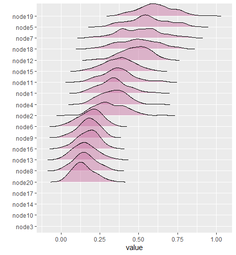
net_stat

#> BGGM: Bayesian Gaussian Graphical Models
#> ---
#> Network Stats: Roll Your Own
#> Posterior Samples: 100
#> ---
#> Estimates:
#>
#>  Node Post.mean Post.sd Cred.lb Cred.ub
#>     1     0.340   0.097   0.166   0.546
#>     2     0.319   0.100   0.176   0.513
#>     3     0.000   0.000   0.000   0.000
#>     4     0.337   0.086   0.189   0.489
#>     5     0.559   0.133   0.332   0.791
#>     6     0.188   0.073   0.029   0.320
#>     7     0.505   0.138   0.241   0.781
#>     8     0.153   0.070   0.022   0.286
#>     9     0.175   0.063   0.041   0.281
#>    10     0.000   0.000   0.000   0.000
#>    11     0.365   0.107   0.178   0.627
#>    12     0.479   0.093   0.280   0.637
#>    13     0.155   0.074   0.022   0.301
#>    14     0.000   0.000   0.000   0.000
#>    15     0.374   0.097   0.175   0.550
#>    16     0.174   0.065   0.034   0.295
#>    17     0.000   0.000   0.000   0.000
#>    18     0.491   0.132   0.238   0.745
#>    19     0.613   0.113   0.408   0.825
#>    20     0.144   0.066   0.038   0.289
#> ---
And then plotted
plot(net_stat)There are additional examples in the documentation.
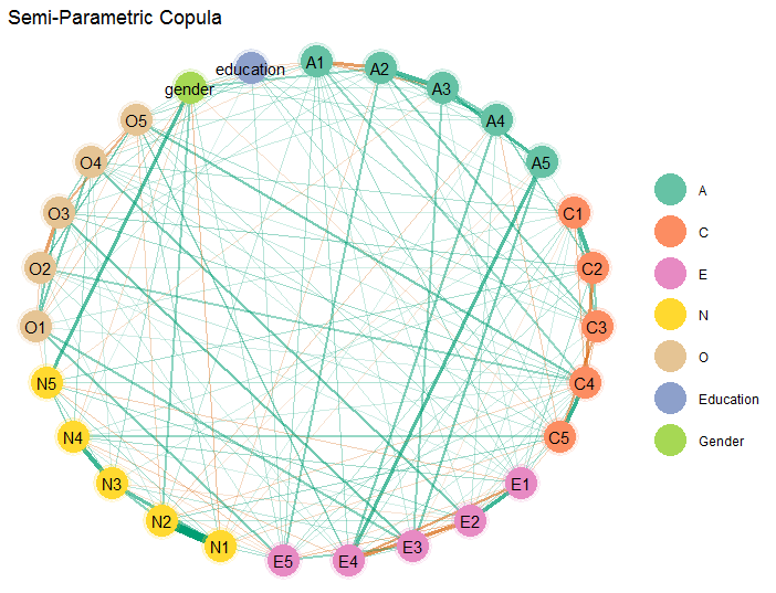
Here is an example of a more involved network plot. In this case, the
graph is estimated with a semi-parametric copula (type = "mixed"),
where two control variables are included in the model.
# personality (includes gender and education)
Y <- bfi

# fit copula GGM
fit <- estimate(Y, type = "mixed")

# select graph
E <- select(fit)
The graph is then plotted
# extract communities
comm <- substring(colnames(Y), 1, 1)

# plot
plot(E,
     # enlarge edges
     edge_magnify = 5,
     # cluster nodes
     groups = comm,
     # change layout
     layout = "circle")$plt +
  # plot title
  ggtitle("Semi-Parametric Copula") +
  # add custom labels
  scale_color_brewer(breaks = c("A", "C",
                                "E", "N",
                                "O", "e",
                                "g"),
                     labels =   c("A", "C",
                                 "E", "N",
                                 "O",
                                 "Education",
                                 "Gender"),
                     palette = "Set2")
Note that layout can be changed to any option provided in the R
package sna (Butts 2019).
The primary focus of BGGM is Gaussian graphical modeling (the inverse covariance matrix). The residue is a suite of useful methods not explicitly for GGMs. For example,
Bivariate correlations for binary (tetrachoric), ordinal
(polychoric), mixed (rank based), and continuous (Pearson’s) data.
Here is an example for computing tetrachoric correlations:
# binary data
Y <- women_math[1:500,]

cors <- zero_order_cors(Y, type = "binary", iter = 250)

cors$R| 1 | 2 | 3 | 4 | 5 | 6 | |
|---|---|---|---|---|---|---|
| 1 | 1.000 | -0.198 | 0.506 | 0.122 | -0.140 | 0.098 |
| 2 | -0.198 | 1.000 | -0.482 | -0.013 | -0.146 | -0.146 |
| 3 | 0.506 | -0.482 | 1.000 | 0.310 | -0.343 | 0.351 |
| 4 | 0.122 | -0.013 | 0.310 | 1.000 | -0.363 | 0.169 |
| 5 | -0.140 | -0.146 | -0.343 | -0.363 | 1.000 | -0.194 |
| 6 | 0.098 | -0.146 | 0.351 | 0.169 | -0.194 | 1.000 |
The object cors also includes the sampled correlation matrices (in
this case 250) in an array.
Multivariate regression for binary (probit), ordinal (probit), mixed (rank likelihood), and continuous data.
Here is an example for a multivariate probit model with an ordinal
outcome, where E5 (“take charge”) and N5 (“panic easily”) are
predicted by gender and education:
# personality data
Y <- bfi

# variables
Y <- subset(Y, select = c("E5", "N5",
                          "gender", "education"))


mv_probit <- estimate(Y, formula = ~ gender + as.factor(education),
                      type = "ordinal")
Note that BGGM does not use the customary model.matrix
formulation. This is for good reason, as each variable in the GGM does
not need to be written out. Here we effectively “tricked” BGGM to
fit a multivariate probit model (each variable included in formula is
removed from Y).
regression_summary(mv_probit)
#> BGGM: Bayesian Gaussian Graphical Models
#> ---
#> Type: ordinal
#> Formula: ~ gender + as.factor(education)
#> ---
#> Coefficients:
#>
#> E5
#>                       Post.mean Post.sd Cred.lb Cred.ub
#> (Intercept)               1.852   0.533   1.049   3.142
#> gender                    0.169   0.066   0.065   0.295
#> as.factor(education)2     0.215   0.109   0.024   0.437
#> as.factor(education)3     0.271   0.104   0.089   0.445
#> as.factor(education)4     0.206   0.103   0.019   0.404
#> as.factor(education)5     0.345   0.128   0.120   0.593
#> ---
#> N5
#>                       Post.mean Post.sd Cred.lb Cred.ub
#> (Intercept)               0.210   0.114  -0.012   0.434
#> gender                    0.502   0.140   0.291   0.835
#> as.factor(education)2    -0.127   0.103  -0.345   0.058
#> as.factor(education)3    -0.104   0.081  -0.258   0.034
#> as.factor(education)4    -0.218   0.104  -0.427  -0.024
#> as.factor(education)5    -0.229   0.103  -0.449  -0.038
#> ---
#> Residual Correlation Matrix:
#>       E5    N5
#> E5  1.00 -0.18
#> N5 -0.18  1.00
#> ---
This basic idea can also be used to fit regression models with a single outcome.
All of the data types (besides continuous) model latent data. That is, unobserved data that is assumed to be Gaussian distributed. For example, a tetrachoric correlation (binary data) is a special case of a polychoric correlation (ordinal data). Both relations are between "theorized normally distributed continuous latent variables Wikepedia. In both instances, the corresponding partial correlation between observed variables is conditioned on the remaining variables in the latent space. This implies that interpretation is similar to continuous data, but with respect to latent variables. We refer interested users to (see page 2364, section 2.2, in Webb and Forster 2008).
BGGM was built specifically for social-behavioral scientists. Of course, the methods can be used by all researchers. However, there is currently not support for high-dimensional data (i.e., more variables than observations) that are common place in, say, the genetics literature. These data are rare in the social-behavioral sciences. In the future, support for high-dimensional data may be added to BGGM.
Bug reports and feature requests can be made by opening an issue on Github. To contribute towards the development of BGGM, you can start a branch with a pull request and we can discuss the proposed changes there.
BGGM is the only R package to implement all of these algorithms
and methods. The mixed data approach is also implemented in the
package sbgcop (base R, Hoff 2007). The R package BDgraph
implements a Gaussian copula graphical model in c++ (Mohammadi and Wit
2015), but not the binary or ordinal approaches. Furthermore, BGGM
is the only package for confirmatory testing and comparing graphical
models with the methods described in Williams et al. (2020).
Albert, James H, and Siddhartha Chib. 1993. “Bayesian Analysis of Binary and Polychotomous Response Data.” Journal of the American Statistical Association 88 (422): 669–79.
Butts, Carter T. 2019. Sna: Tools for Social Network Analysis. https://CRAN.R-project.org/package=sna.
Chu, Jen-hwa, Scott T Weiss, Vincent J Carey, and Benjamin A Raby. 2009. “A Graphical Model Approach for Inferring Large-Scale Networks Integrating Gene Expression and Genetic Polymorphism.” BMC Systems Biology 3 (1): 55.
Cowles, Mary Kathryn. 1996. “Accelerating Monte Carlo Markov Chain Convergence for Cumulative-Link Generalized Linear Models.” Statistics and Computing 6 (2): 101–11.
Eddelbuettel, Dirk, Romain François, J Allaire, Kevin Ushey, Qiang Kou, N Russel, John Chambers, and D Bates. 2011. “Rcpp: Seamless R and C++ Integration.” Journal of Statistical Software 40 (8): 1–18.
Gelman, Andrew, Ben Goodrich, Jonah Gabry, and Aki Vehtari. 2019. “R-squared for Bayesian Regression Models.” American Statistician 73 (3): 307–9. https://doi.org/10.1080/00031305.2018.1549100.
Gelman, Andrew, Xiao-Li Meng, and Hal Stern. 1996. “Posterior predictive assessment of model fitness via realized discrepancies. Vol.6, No.4.” Statistica Sinica 6 (4): 733–807. https://doi.org/10.1.1.142.9951.
Haslbeck, Jonas MB, and Lourens J Waldorp. 2018. “How Well Do Network Models Predict Observations? On the Importance of Predictability in Network Models.” Behavior Research Methods 50 (2): 853–61.
Hoff, Peter D. 2007. “Extending the Rank Likelihood for Semiparametric Copula Estimation.” The Annals of Applied Statistics 1 (1): 265–83.
Hoijtink, H. 2011. Informative hypotheses: Theory and practice for behavioral and social scientists. Chapman; Hall/CRC.
Jeffreys, Harold. 1961. The theory of probability. Oxford: Oxford University Press.
Jones, Payton J, Ruofan Ma, and Richard J McNally. 2019. “Bridge Centrality: A Network Approach to Understanding Comorbidity.” Multivariate Behavioral Research, 1–15.
Kass, Robert E, and Adrian E Raftery. 1995. “Bayes Factors.” Journal of the American Statistical Association 90 (430): 773–95.
Lawrence, Earl, Derek Bingham, Chuanhai Liu, and Vijayan N Nair. 2008. “Bayesian Inference for Multivariate Ordinal Data Using Parameter Expansion.” Technometrics 50 (2): 182–91.
Millington, Tristan, and Mahesan Niranjan. 2020. “Partial Correlation Financial Networks.” Applied Network Science 5 (1): 11.
Mohammadi, Reza, and Ernst C Wit. 2015. “BDgraph: An R Package for Bayesian Structure Learning in Graphical Models.” arXiv Preprint arXiv:1501.05108.
Mulder, Joris, Xin Gu, Anton Olsson-Collentine, Andrew Tomarken, Florian Böing-Messing, Herbert Hoijtink, Marlyne Meijerink, et al. 2019. “BFpack: Flexible Bayes Factor Testing of Scientific Theories in R.” arXiv Preprint arXiv:1911.07728.
Mulder, Joris, and Luis Pericchi. 2018. “The Matrix-F Prior for Estimating and Testing Covariance Matrices.” Bayesian Analysis, no. 4: 1–22. https://doi.org/10.1214/17-BA1092.
Rodriguez, Josue E, Donald R Williams, Philippe Rast, and Joris Mulder. 2020. “On Formalizing Theoretical Expectations: Bayesian Testing of Central Structures in Psychological Networks.” PsyArXiv.
Rubin, Donald B. 1984. “Bayesianly Justifiable and Relevant Frequency Calculations for the Applied Statistician.” The Annals of Statistics, 1151–72.
Sanderson, Conrad, and Ryan Curtin. 2016. “Armadillo: A Template-Based C++ Library for Linear Algebra.” Journal of Open Source Software 1 (2): 26.
Talhouk, Aline, Arnaud Doucet, and Kevin Murphy. 2012. “Efficient Bayesian Inference for Multivariate Probit Models with Sparse Inverse Correlation Matrices.” Journal of Computational and Graphical Statistics 21 (3): 739–57.
Webb, Emily L, and Jonathan J Forster. 2008. “Bayesian Model Determination for Multivariate Ordinal and Binary Data.” Computational Statistics & Data Analysis 52 (5): 2632–49.
Williams, Donald R. 2018. “Bayesian Estimation for Gaussian Graphical Models: Structure Learning, Predictability, and Network Comparisons.” arXiv. https://doi.org/10.31234/OSF.IO/X8DPR.
Williams, Donald R, and Joris Mulder. 2019. “Bayesian Hypothesis Testing for Gaussian Graphical Models: Conditional Independence and Order Constraints.” PsyArXiv. https://doi.org/10.31234/osf.io/ypxd8.
Williams, Donald R, Philippe Rast, Luis R Pericchi, and Joris Mulder. 2020. “Comparing Gaussian Graphical Models with the Posterior Predictive Distribution and Bayesian Model Selection.” Psychological Methods.
Zerenner, Tanja, Petra Friederichs, Klaus Lehnertz, and Andreas Hense. 2014. “A Gaussian Graphical Model Approach to Climate Networks.” Chaos: An Interdisciplinary Journal of Nonlinear Science 24 (2): 023103.
