zooper

An R package to download and integrate zooplankton data from the Sacramento San Joaquin Delta.

Installation

You can install the latest version from R-universe with:

options(repos = c(
    sbashevkin = 'https://sbashevkin.r-universe.dev',
    CRAN = 'https://cloud.r-project.org'))

install.packages(“zooper”)

Or from GitHub with:

# install.packages("devtools")
devtools::install_github("InteragencyEcologicalProgram/zooper")

Dataset documentation

For a full documentation of this dataset please see the data paper in PLOS ONE or the data publication on EDI

Bashevkin, S. M., R. Hartman, M. Thomas, A. Barros, C. E. Burdi, A. Hennessy, T. Tempel, and K. Kayfetz. 2022. Five decades (1972–2020) of zooplankton monitoring in the upper San Francisco Estuary. PLOS ONE 17: e0265402. doi:10.1371/journal.pone.0265402

Bashevkin, S. M., R. Hartman, M. Thomas, A. Barros, C. Burdi, A. Hennessy, T. Tempel, K. Kayfetz, K. Alstad, and C. Pien. 2023. Interagency Ecological Program: Zooplankton abundance in the Upper San Francisco Estuary from 1972-2021, an integration of 7 long-term monitoring programs. ver 4. Environmental Data Initiative. doi:10.6073/pasta/8b646dfbeb625e308212a39f1e46f69b

Introduction

This package has 2 main functions and a few accessory functions. The Zoopdownloader function downloads the zooplankton datasets from their respective online sources and converts them to a consistent format. The Zoopsynther function takes zooplankton data from different surveys and integrates the data according to user-specified parameter choices.

This package is also accessible through a shiny app (code and installation instructions for latest version available here). The app is a GUI (graphical user interface) that allows users without R experience to run the zooplankton synthesizer function and download the resulting data. The shiny app also allows users with all experience levels to easily visualize the data.

Community or taxon-specific analyses?

The biggest problem with integrating zooplankton datasets is variability in taxonomic resolution. To resolve this, we have developed 2 approaches to consolidating inconsistent data to “least common denominator taxa.” Depending on what type of analysis you wish to run, you may wish for different types of synthesized data.

For community data analyzers

I want to analyze the community composition at whatever taxonomic level lets me use all these datasets.

Consistent taxonomic categories
No plankters counted more than once
Sacrifices some taxonomic resolution
Removes taxa with no relatives in all datasets (e.g., Annelida)

For specific taxa analyzers

I want all possible data on these specific taxa.

Calculates total CPUE for higher taxonomic levels
Some plankters appear in multiple nested taxa (e.g., Calanoida, Copepoda)
Preserves taxonomic resolution and creates taxonomic categories that are comparable across all datasets
Labels taxa that are comparable across all datasets, warns about those that are not.

Size classes

We have integrated zooplankton data from 3 net size classes:

Macro (500 - 505 μm): Amphipods and mysids (NOTE: Prior to 1974 EMP macrozooplankton were sampled with a 930 μm mesh net)
Meso (150 - 160 μm): Copepods, cladocera
Micro (43 - 50 μm): Copepods, rotifers

Nets accurately sample zooplankton larger than the mesh size. Zooplankton smaller than the mesh size are still captured and often recorded in datasets, but the resulting CPUEs are not accurate. To account for this we:

Resolve taxonomic resolution separately within each net size class.
If Data = 'Taxa', we mark “summed groups” with the net size class from which they were derived.
All potentially undersampled data are marked with a flag Undersampled == TRUE
For the plots in the shiny app, all data with Undersampled == TRUE can be removed. However, data downloaded from the app do contain undersampled data.

Changing taxonomic resolution over time

For many studies, taxonomic resolution has changed over time. This could confound analyses of zooplankton communities and abundances over time. To account for this, we have implemented a solution for the Data_type="Community" option, which can be implemented by setting Time_consistency = TRUE.

We first find all taxa that were not counted every year across the date range the user inputs (but taking into account the years non-native species were introduced and each survey first started sampling). These taxa are then summed to higher taxonomic levels, as is done for taxa that were not counted across all datasets.

Often, non-native species are not added to zooplankton species list the same year they are first detected in the system. To allow for some lag between introduction years and the years these species were first counted, you can change the Intro_lag option (currently defaults to 2 years).

Biomass

Functionality to output biomass (carbon biomass per unit effort in $\mu g$ $m^{-3}$) is now included in zooper. However, biomass conversions are not available for all taxa and life stages. Micro and meso zooplankton are converted to biomass using average biomass values from the literature (see biomass_mesomicro for sources). The macrozooplankton are converted to biomass using length-weight equations (see biomass_macro for sources). Length data are currently only published online for EMP, so only EMP macro zooplankton biomass is available through zooper, and only for the two mysid taxa with dry weight length-weight equations from formalin preserved specimens (see biomass_macro for the full set of equations). As more conversions become available for any size class, they can be added to zooper to increase the biomass coverage.

Usage

library(zooper)
MyZoops <- Zoopsynther(Data_type = "Community", 
                       Response = c("CPUE", "BPUE"),
                       Sources = c("EMP", "FRP", "FMWT"), 
                       Size_class = "Meso", 
                       Date_range = c("1990-10-01", "2000-09-30"))
#> [1] "No disclaimers here! Enjoy the clean data!"

str(MyZoops)
#> tibble [151,478 × 36] (S3: tbl_df/tbl/data.frame)
#>  $ Source      : chr [1:151478] "EMP" "EMP" "EMP" "EMP" ...
#>  $ SizeClass   : chr [1:151478] "Meso" "Meso" "Meso" "Meso" ...
#>  $ Volume      : num [1:151478] 10.6 10.6 10.6 10.6 10.6 ...
#>  $ Lifestage   : chr [1:151478] "Adult" "Adult" "Adult" "Adult" ...
#>  $ Taxname     : chr [1:151478] "Acanthocyclops_UnID" "Acartia_UnID" "Acartiella sinensis" "Asplanchna_UnID" ...
#>  $ Phylum      : chr [1:151478] "Arthropoda" "Arthropoda" "Arthropoda" "Rotifera" ...
#>  $ Class       : chr [1:151478] "Copepoda" "Copepoda" "Copepoda" "Eurotatoria" ...
#>  $ Order       : chr [1:151478] "Cyclopoida" "Calanoida" "Calanoida" "Ploima" ...
#>  $ Family      : chr [1:151478] "Cyclopidae" "Acartiidae" "Acartiidae" "Asplanchnidae" ...
#>  $ Genus       : chr [1:151478] "Acanthocyclops" "Acartia" "Acartiella" "Asplanchna" ...
#>  $ Species     : chr [1:151478] NA NA "Acartiella sinensis" NA ...
#>  $ Taxlifestage: chr [1:151478] "Acanthocyclops_UnID Adult" "Acartia_UnID Adult" "Acartiella sinensis Adult" "Asplanchna_UnID Adult" ...
#>  $ SampleID    : chr [1:151478] "EMP NZEZ2 1994-03-21" "EMP NZEZ2 1994-03-21" "EMP NZEZ2 1994-03-21" "EMP NZEZ2 1994-03-21" ...
#>  $ CPUE        : num [1:151478] 11.34 1.89 5.67 0 0 ...
#>  $ BPUE        : num [1:151478] 0.3176 0.2821 0.252 0.0284 0.0567 ...
#>  $ Undersampled: logi [1:151478] FALSE FALSE FALSE TRUE FALSE FALSE ...
#>  $ Date        : POSIXct[1:151478], format: "1994-03-21" "1994-03-21" ...
#>  $ Station     : chr [1:151478] "NZEZ2" "NZEZ2" "NZEZ2" "NZEZ2" ...
#>  $ Chl         : num [1:151478] NA NA NA NA NA NA NA NA NA NA ...
#>  $ Secchi      : num [1:151478] 35 35 35 35 35 35 35 35 35 35 ...
#>  $ Temperature : num [1:151478] 14.8 14.8 14.8 14.8 14.8 14.8 14.8 14.8 14.8 14.8 ...
#>  $ BottomDepth : num [1:151478] NA NA NA NA NA NA NA NA NA NA ...
#>  $ Tide        : chr [1:151478] "High slack" "High slack" "High slack" "High slack" ...
#>  $ TowType     : chr [1:151478] "Oblique" "Oblique" "Oblique" "Oblique" ...
#>  $ Datetime    : POSIXct[1:151478], format: "1994-03-21 09:25:00" "1994-03-21 09:25:00" ...
#>  $ TurbidityNTU: num [1:151478] NA NA NA NA NA NA NA NA NA NA ...
#>  $ pH          : num [1:151478] NA NA NA NA NA NA NA NA NA NA ...
#>  $ DO          : num [1:151478] NA NA NA NA NA NA NA NA NA NA ...
#>  $ Microcystis : chr [1:151478] NA NA NA NA ...
#>  $ Year        : num [1:151478] 1994 1994 1994 1994 1994 ...
#>  $ TurbidityFNU: num [1:151478] NA NA NA NA NA NA NA NA NA NA ...
#>  $ AmphipodCode: chr [1:151478] NA NA NA NA ...
#>  $ SalSurf     : num [1:151478] 0.644 0.644 0.644 0.644 0.644 ...
#>  $ SalBott     : num [1:151478] 0.958 0.958 0.958 0.958 0.958 ...
#>  $ Latitude    : num [1:151478] NA NA NA NA NA NA NA NA NA NA ...
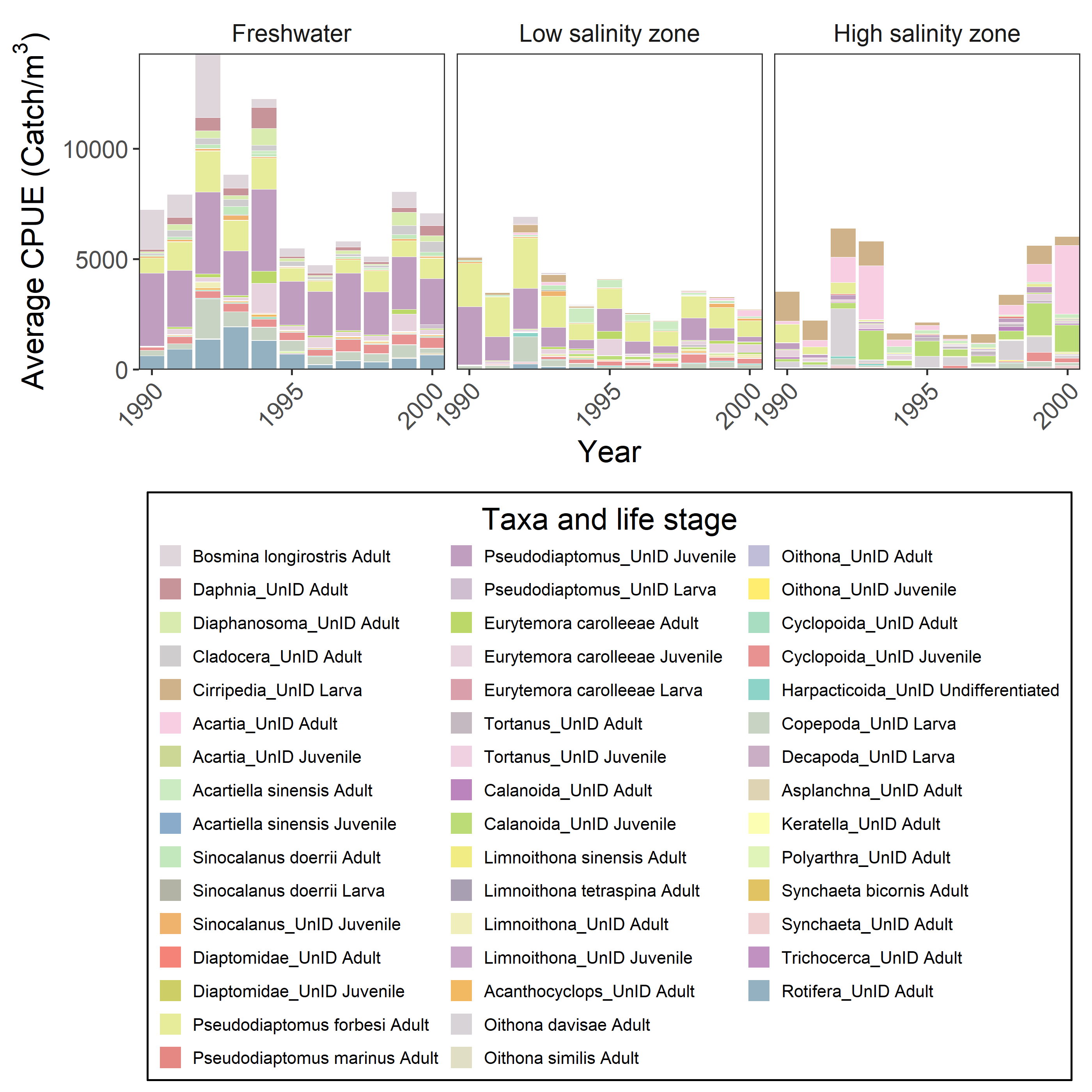
#>  $ Longitude   : num [1:151478] NA NA NA NA NA NA NA NA NA NA ...

Here’s a graph you could make with the data

library(dplyr)
library(ggplot2)
library(RColorBrewer)
set.seed(16)

MyZoops%>%
  filter(!is.na(SalSurf))%>%
  mutate(Salinity_zone=case_when(
    SalSurf < 0.5 ~ "Freshwater",
    SalSurf > 0.5 & SalSurf < 6 ~ "Low salinity zone",
    SalSurf > 6 ~ "High salinity zone"
  ))%>%
  mutate(Salinity_zone=factor(Salinity_zone, levels=c("Freshwater", "Low salinity zone", "High salinity zone")))%>%
  group_by(Year,Phylum, Class, Order, Family, Genus, Species, Lifestage, Taxlifestage, Salinity_zone)%>%
  summarise(CPUE=mean(CPUE, na.rm=T), .groups="drop")%>%
  arrange(Phylum, Class, Order, Family, Genus, Species, Lifestage)%>%
  mutate(Taxlifestage=factor(Taxlifestage, unique(Taxlifestage)))%>%
  ggplot(aes(x=Year, y=CPUE))+
  geom_bar(stat="identity", color="white", linewidth=0.01, aes(fill=Taxlifestage))+
  facet_wrap(~Salinity_zone, nrow=1)+
  coord_cartesian(expand=0)+
  scale_x_continuous(breaks = function(x) unique(floor(pretty(seq(min(x), max(x)), n=3))), expand=c(0,0))+
  scale_fill_manual(values=sample(colorRampPalette(brewer.pal(12, "Set3"))(length(unique(MyZoops$Taxlifestage)))), 
                    name="Taxa and life stage", 
                    guide = guide_legend(ncol=3, title.position = "top", title.hjust = 0.5))+
  ylab(bquote(Average~CPUE~"("*Catch*"/"*m^3*")"))+
  theme_bw()+
  theme(panel.grid=element_blank(), text=element_text(size=14), legend.text = element_text(size=8), 
        legend.key.size = unit(10, "points"), strip.background=element_blank(), legend.position = "bottom", 
        legend.background = element_rect(color="black"), axis.text.x=element_text(angle=45, hjust=1))

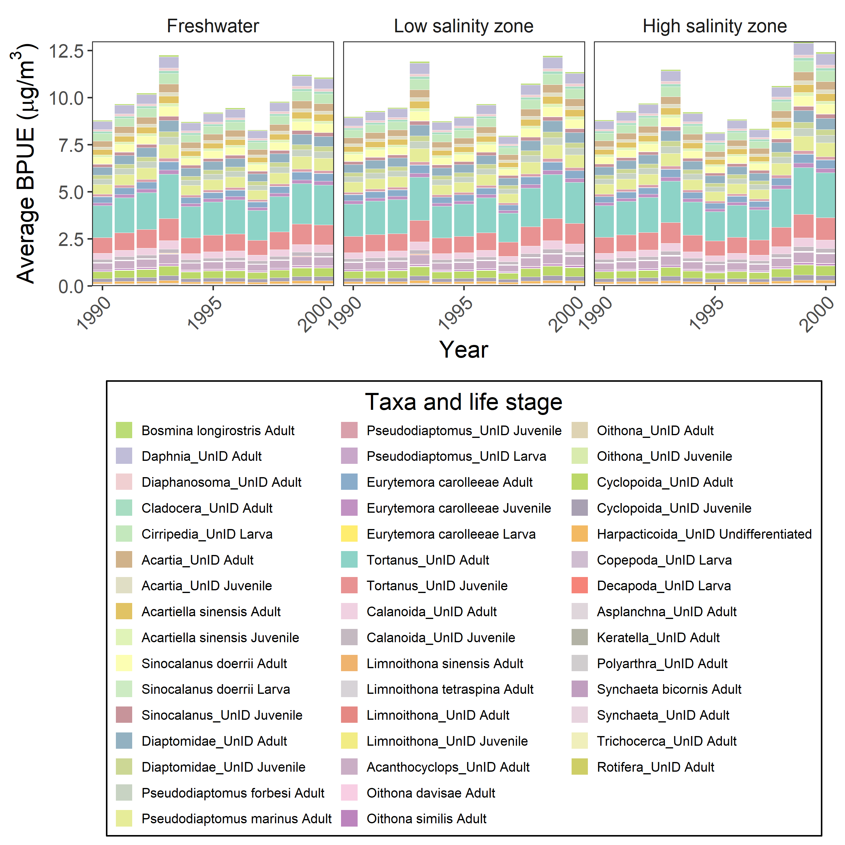
Here’s the same graph with biomass (although a few taxa were removed for which biomass conversions were not available)

MyZoops%>%
  filter(!is.na(SalSurf))%>%
  mutate(Salinity_zone=case_when(
    SalSurf < 0.5 ~ "Freshwater",
    SalSurf > 0.5 & SalSurf < 6 ~ "Low salinity zone",
    SalSurf > 6 ~ "High salinity zone"
  ))%>%
  mutate(Salinity_zone=factor(Salinity_zone, levels=c("Freshwater", "Low salinity zone", "High salinity zone")))%>%
  group_by(Year,Phylum, Class, Order, Family, Genus, Species, Lifestage, Taxlifestage, Salinity_zone)%>%
  summarise(BPUE=mean(BPUE, na.rm=T), .groups="drop")%>%
  arrange(Phylum, Class, Order, Family, Genus, Species, Lifestage)%>%
  mutate(Taxlifestage=factor(Taxlifestage, unique(Taxlifestage)))%>%
  ggplot(aes(x=Year, y=BPUE))+
  geom_bar(stat="identity", color="white", linewidth=0.01, aes(fill=Taxlifestage))+
  facet_wrap(~Salinity_zone, nrow=1)+
  coord_cartesian(expand=0)+
  scale_x_continuous(breaks = function(x) unique(floor(pretty(seq(min(x), max(x)), n=3))), expand=c(0,0))+
  scale_fill_manual(values=sample(colorRampPalette(brewer.pal(12, "Set3"))(length(unique(MyZoops$Taxlifestage)))), 
                    name="Taxa and life stage", 
                    guide = guide_legend(ncol=3, title.position = "top", title.hjust = 0.5))+
  ylab(bquote(Average~BPUE~"("*mu*g*"/"*m^3*")"))+
  theme_bw()+
  theme(panel.grid=element_blank(), text=element_text(size=14), legend.text = element_text(size=8), 
        legend.key.size = unit(10, "points"), strip.background=element_blank(), legend.position = "bottom", 
        legend.background = element_rect(color="black"), axis.text.x=element_text(angle=45, hjust=1))

Code of conduct

Please note that the ‘zooper’ project is released with a Contributor Code of Conduct. By contributing to this project, you agree to abide by its terms.