cd ~/git_repos
git clone https://github.com/IoannisKaragiannis/brain_tumor_classifier.git

cd brain_tumor_classifier
chmod +x setup_env.sh
chmod +x remove_env.sh

./setup_env.sh

source ~/python_venv/brain/bin/activate
Download the dataset from here and extract them inside this repo under the name brain_tumor_mri_dataset.
Perform data exploration
(brain)$ python3 src/data_exploration.py
The results will be stored under the report/img directory.
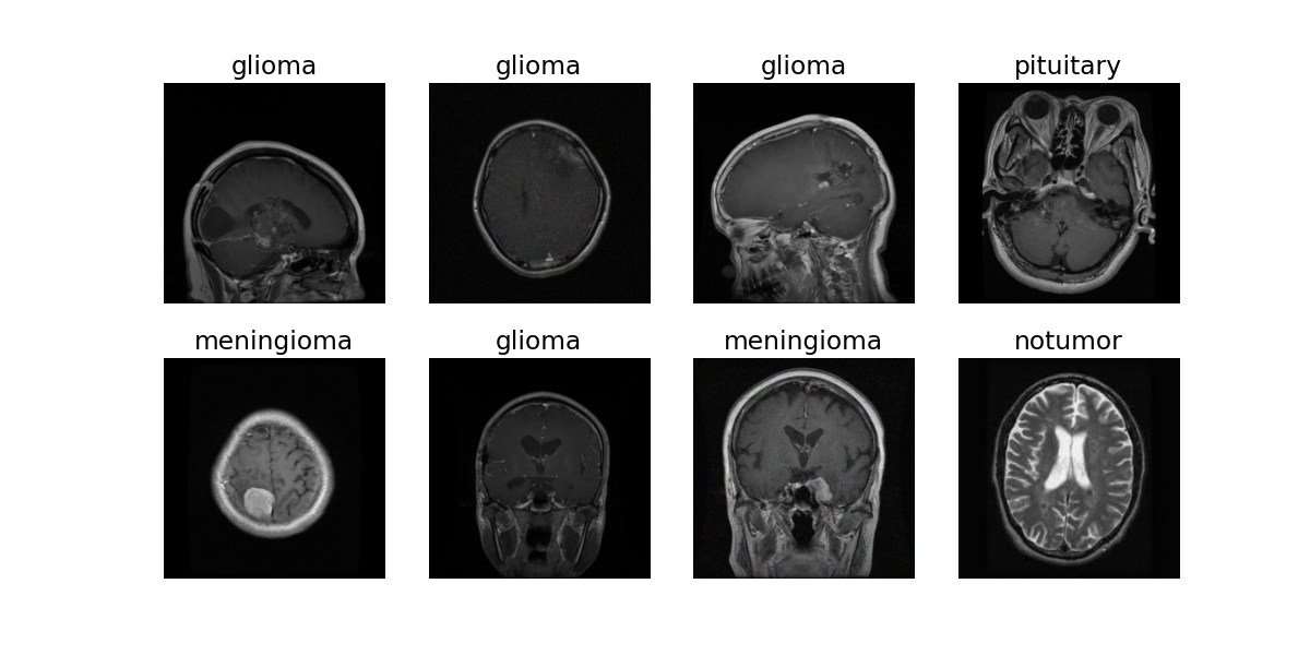
Below you can see an example of some random training data:
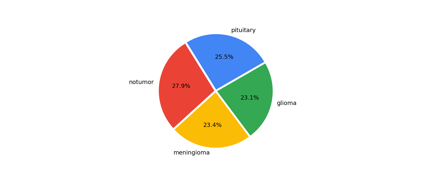
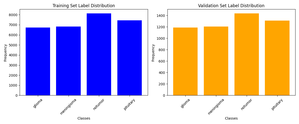
We can also observe that the training data are quite balanced
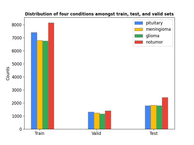
Below one can observe that the distribution of the four different classes, namely glioma, meningioma, notumor, and pituitary is balanced among the training, validation and test data.
-
Download the MRI data from here.
-
Unzip the file and copy it in the root directory of the current repo under the name
brain_tumor_mri_dataset -
Rename the subdirectories into
trainandtestaccordingly. -
The data have different dimensions. For convenience while performing data augmentation I also resize them to 256x256.
-
To perform data augmentation do the following. You can add more augmentation techniques but be cautious when it comes to MRI dataset. If the distribution of the augmented dataset diverges significantly then the model will learn erroneously.
# augment train data
(brain)$ python3 src/augment_data.py --data train

# augment test data
(brain)$ python3 src/augment_data.py --data test
It will take a while. Next to the
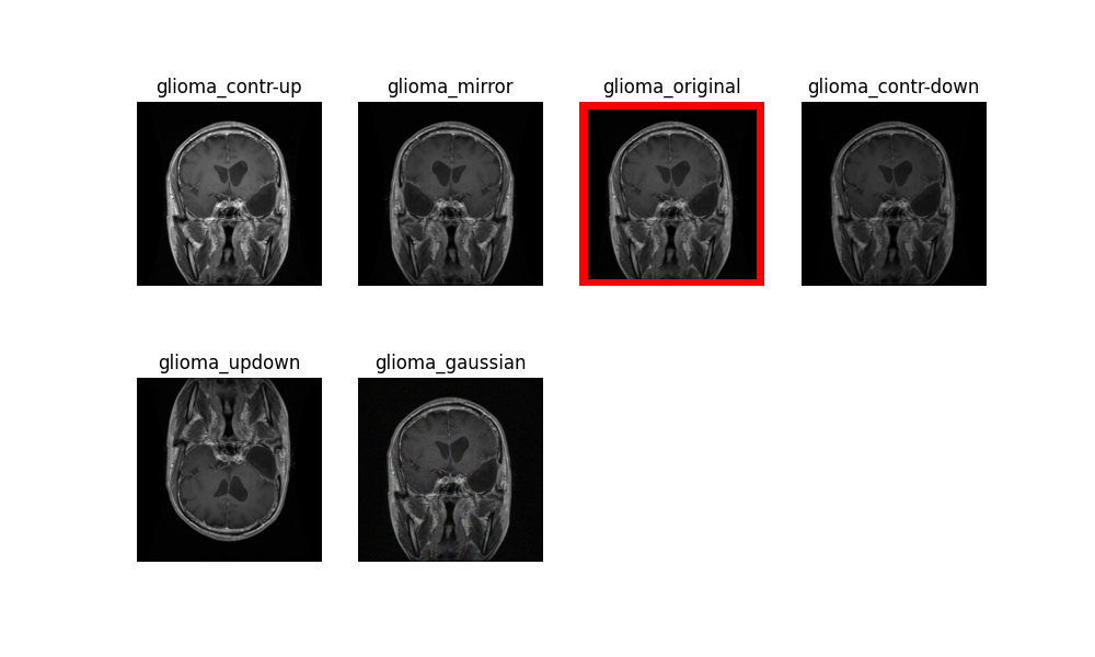
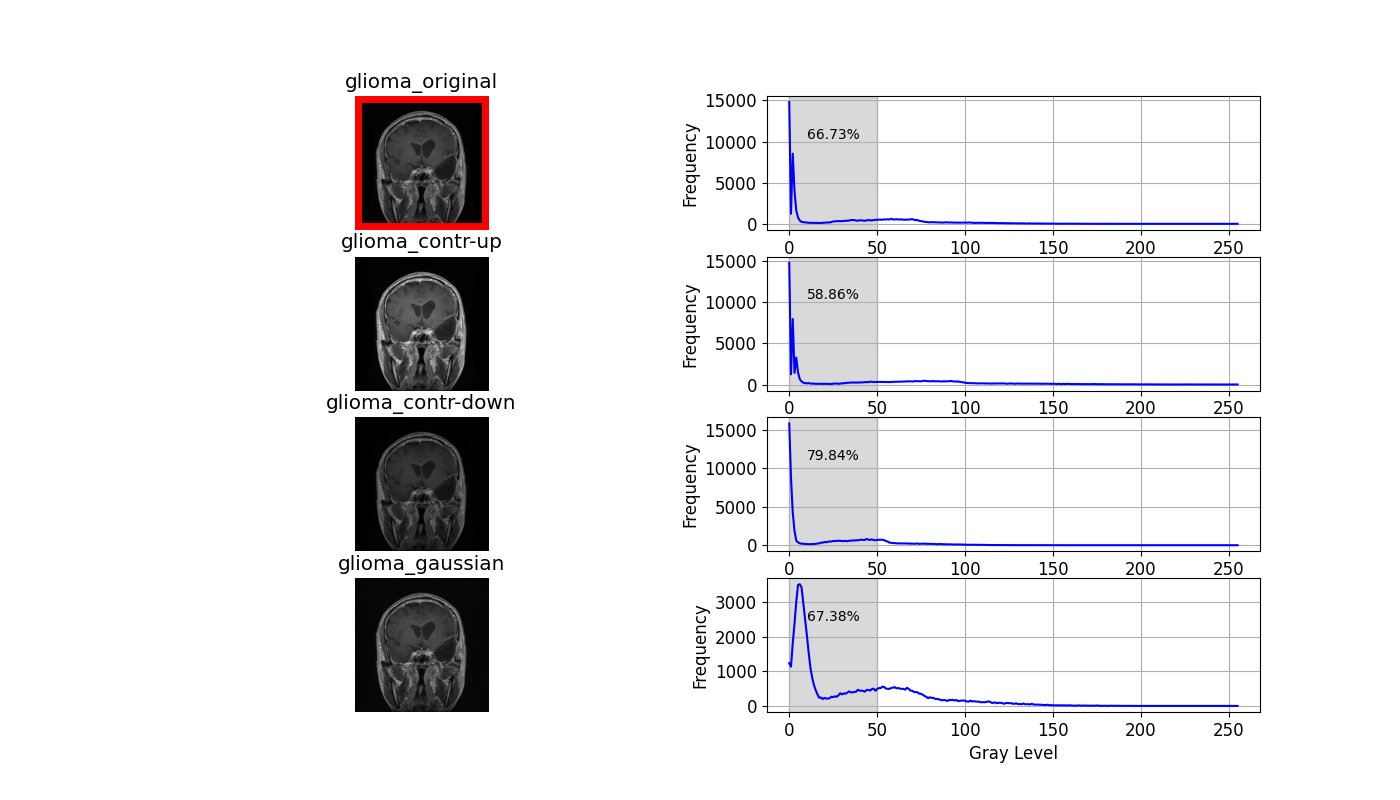
trainandtestfolders, a new directory calledtrain_augmentedortest_augmentedwill be created accordingly. Only the training data or their augmented version will be used throughout the training process while the test data will be left untouched for evaluation purposes. An example of the different augmentation techniques applied on one particular glioma sample:
The three augmentation techniques directly affecting the histogram of the original image are shown below.
In the context of MRI images, the predominant composition comprises low-intensity pixels, shaping a left-skewed histogram. To compare these histograms, I've highlighted the dark regions, particularly those below an intensity of 50. Observations on contrast adjustments reveal a reduction in dark region pixel percentage from 66.73% to 58.86% with increased contrast and vice versa with decreased contrast.
Contrast adjustments influence pixel distribution within the dark region, yet gaussian blurring exhibits minimal impact on the percentage of dark pixels. However, it does alter the distribution pattern within this darker range.
In an effort to eliminate the dark background I tried to crop the image. However, I ended up losing vital brain structures. Retaining the dark background, inherent in all MRI images, appears judicious, allowing the classifier to discern its insignificance.
My experience underscores the necessity of comprehending the impact of data augmentation on MRI images. Verifying whether the augmented version remains representative of the original image is crucial. Seeking input from medical experts stands as an indispensable step in this process.
# test single image (modify the test_sample and test_label in the config.ini)
(brain)$ python3 src/test_single_mri.py

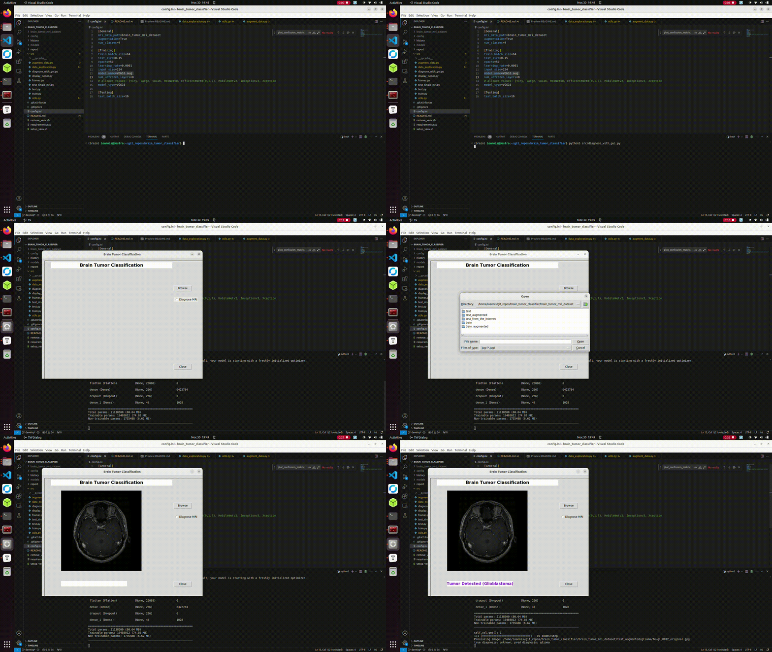
# test single image with GUI
(brain)$ python3 src/diagnose_with_gui.py

# evaluate model on test-set
(brain)$ python3 src/test.py
Below you will find the performance of 4 different models, with and without data augmentation.
[General]
mri_data_path=brain_tumor_mri_dataset
augmentation=False
num_classes=4

[Training]
train_batch_size=32
test_size=0.2
epochs=50
learning_rate=0.0001
input_size=224
model_name=ResNet50
num_unfrozen_layers=9
# allowed values: {tiny, large, VGG16, ResNet50, EfficientNetB{0,1,7}, MobileNetv2, Inceptionv3, Xception
model_type=ResNet50

[Testing]
test_batch_size=16
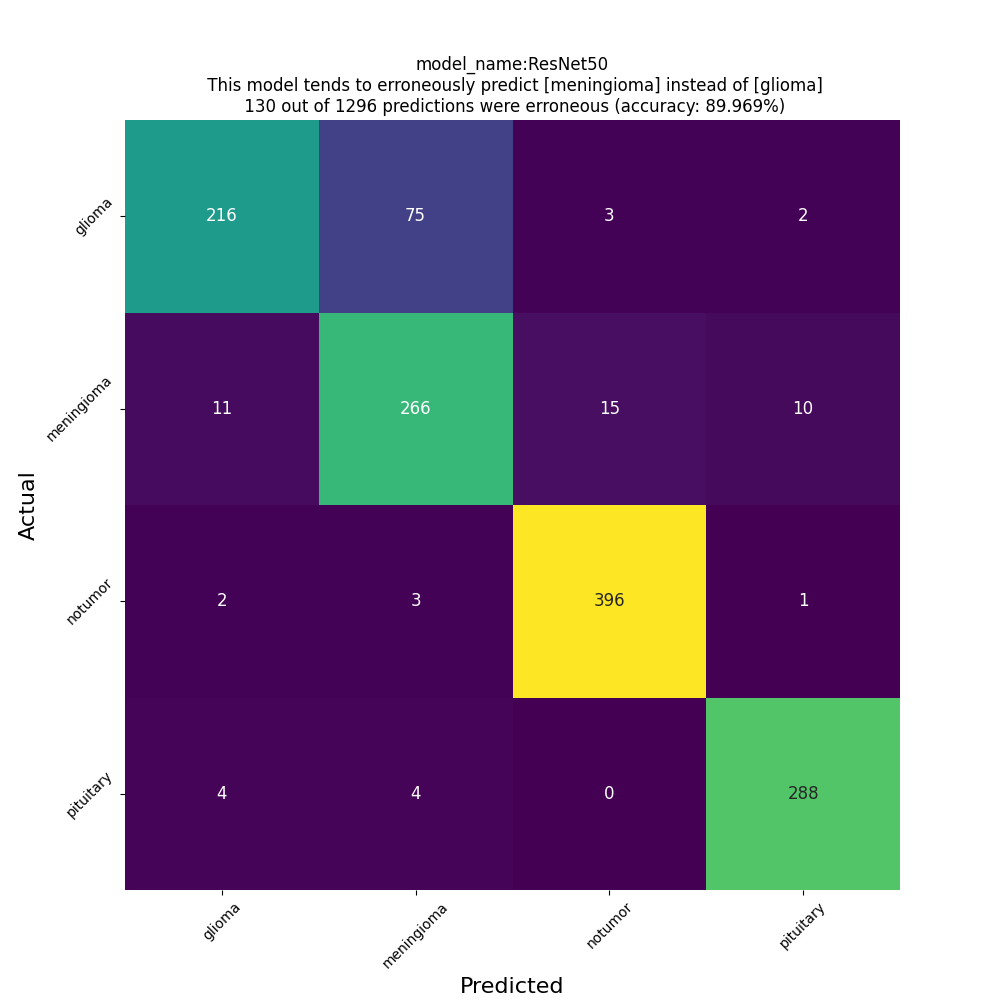
classification report
Test Loss: 0.3312033712863922
Test Accuracy: 0.8996913433074951
Predicting for 1296 samples
81/81 [==============================] - 121s 1s/step
QSocketNotifier: Can only be used with threads started with QThread
Classification Report:
              precision    recall  f1-score   support

      glioma       0.93      0.73      0.82       296
  meningioma       0.76      0.88      0.82       302
     notumor       0.96      0.99      0.97       402
   pituitary       0.96      0.97      0.96       296

    accuracy                           0.90      1296
   macro avg       0.90      0.89      0.89      1296
weighted avg       0.91      0.90      0.90      1296
confusion matrix
[General]
mri_data_path=brain_tumor_mri_dataset
augmentation=True
num_classes=4

[Training]
train_batch_size=64
test_size=0.15
epochs=50
learning_rate=0.0001
input_size=224
model_name=ResNet50_aug
num_unfrozen_layers=15
# allowed values: {tiny, large, VGG16, ResNet50, EfficientNetB{0,1,7}, MobileNetv2, Inceptionv3, Xception
model_type=ResNet50

[Testing]
test_batch_size=16
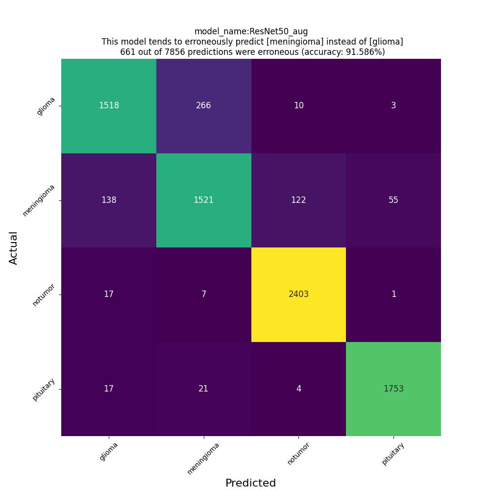
classification report
Test Loss: 0.3191703259944916
Test Accuracy: 0.9158604741096497
Predicting for 7856 samples
491/491 [==============================] - 709s 1s/step
QSocketNotifier: Can only be used with threads started with QThread
Classification Report:
              precision    recall  f1-score   support

      glioma       0.90      0.84      0.87      1797
  meningioma       0.84      0.83      0.83      1836
     notumor       0.95      0.99      0.97      2428
   pituitary       0.97      0.98      0.97      1795

    accuracy                           0.92      7856
   macro avg       0.91      0.91      0.91      7856
weighted avg       0.91      0.92      0.92      7856
confusion matrix
[General]
mri_data_path=brain_tumor_mri_dataset
augmentation=False
num_classes=4

[Training]
train_batch_size=32
test_size=0.2
epochs=50
learning_rate=0.0001
input_size=224
model_name=VGG16
num_unfrozen_layers=4
# allowed values: {tiny, large, VGG16, ResNet50, EfficientNetB{0,1,7}, MobileNetv2, Inceptionv3, Xception
model_type=VGG16

[Testing]
test_batch_size=16
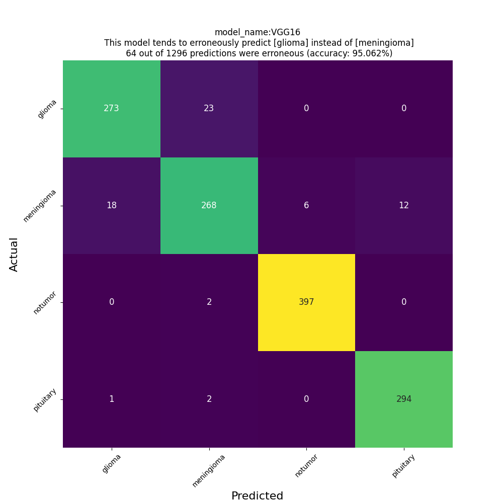
classification report
Test Loss: 0.20448878407478333
Test Accuracy: 0.9506173133850098
Predicting for 1296 samples
81/81 [==============================] - 2s 24ms/step
Classification Report:
              precision    recall  f1-score   support

      glioma       0.93      0.92      0.93       296
  meningioma       0.91      0.88      0.89       304
     notumor       0.99      1.00      0.99       401
   pituitary       0.96      0.99      0.97       295

    accuracy                           0.95      1296
   macro avg       0.95      0.95      0.95      1296
weighted avg       0.95      0.95      0.95      1296
confusion matrix
[General]
mri_data_path=brain_tumor_mri_dataset
augmentation=True
num_classes=4

[Training]
train_batch_size=64
test_size=0.15
epochs=50
learning_rate=0.0001
input_size=224
model_name=VGG16_aug
num_unfrozen_layers=8
# allowed values: {tiny, large, VGG16, ResNet50, EfficientNetB{0,1,7}, MobileNetv2, Inceptionv3, Xception
model_type=VGG16

[Testing]
test_batch_size=16
It is worth mentioning that throughout the training process, when splitting the training and validation data I maintained the proportion of classes in both the training and validation datasets (having the same class distribution) by using the stratify variable. This is what the train and valid data look like.
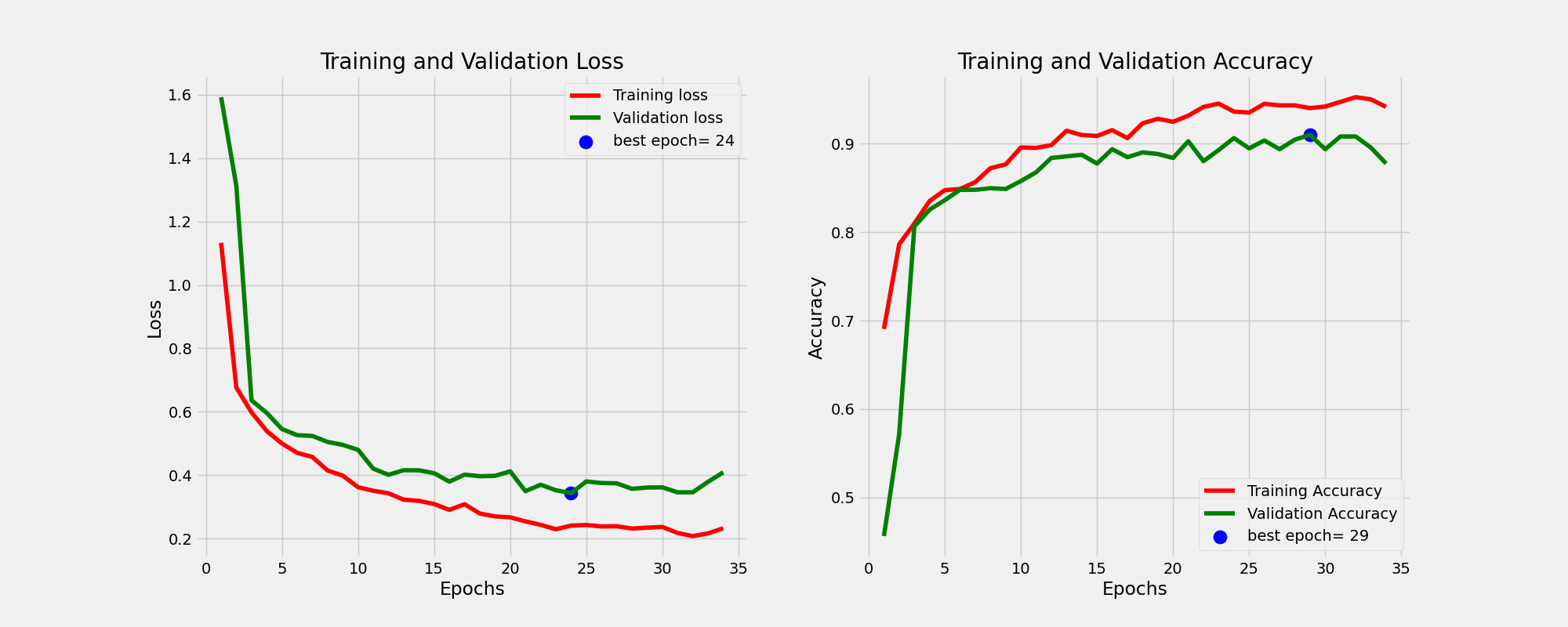
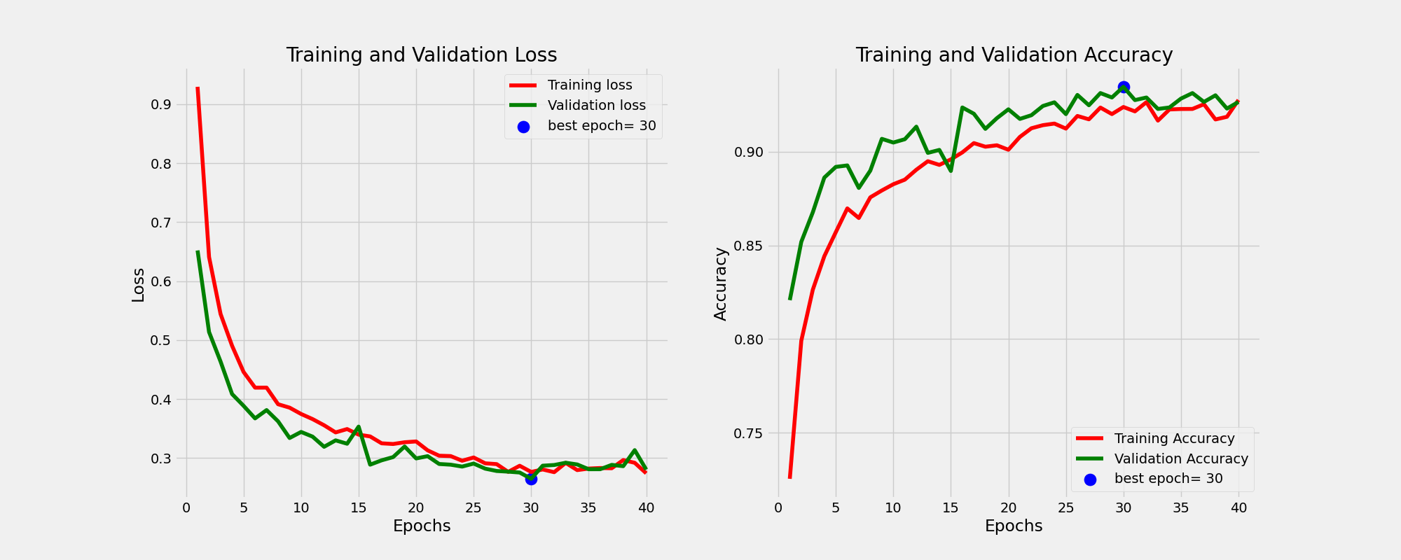
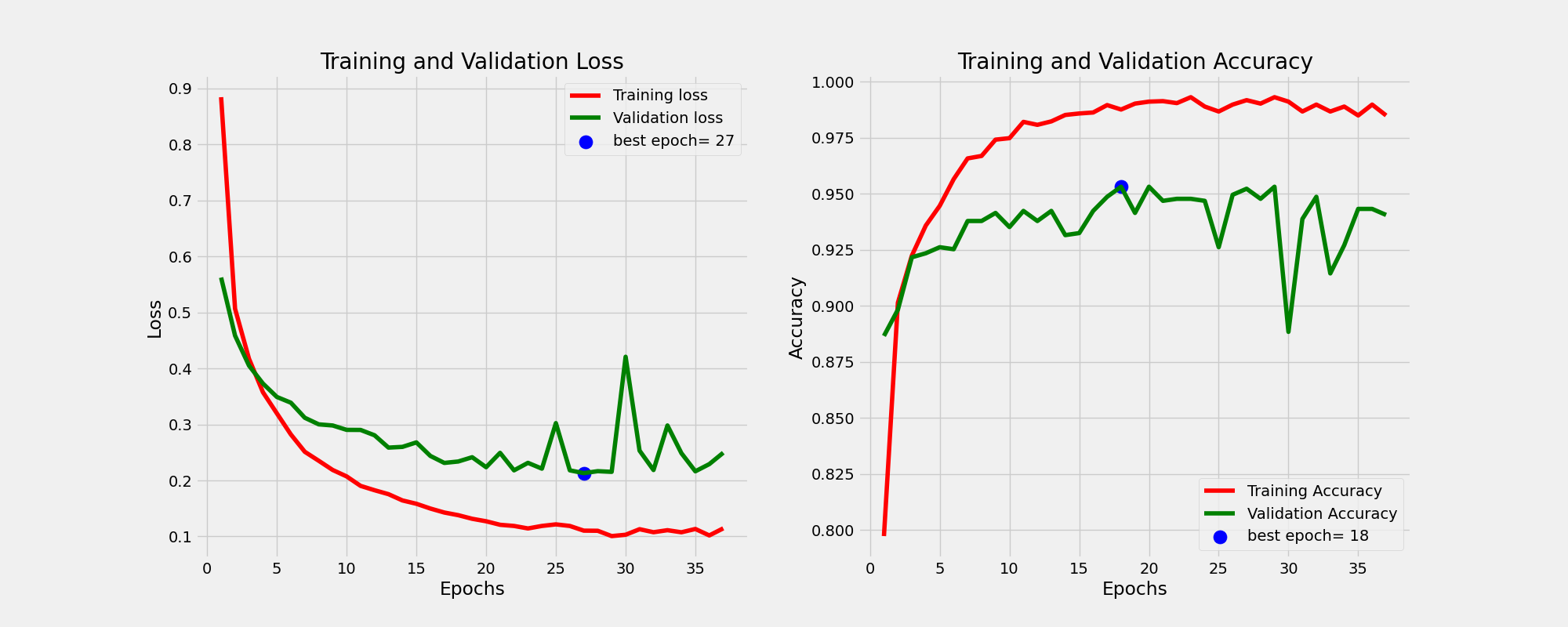
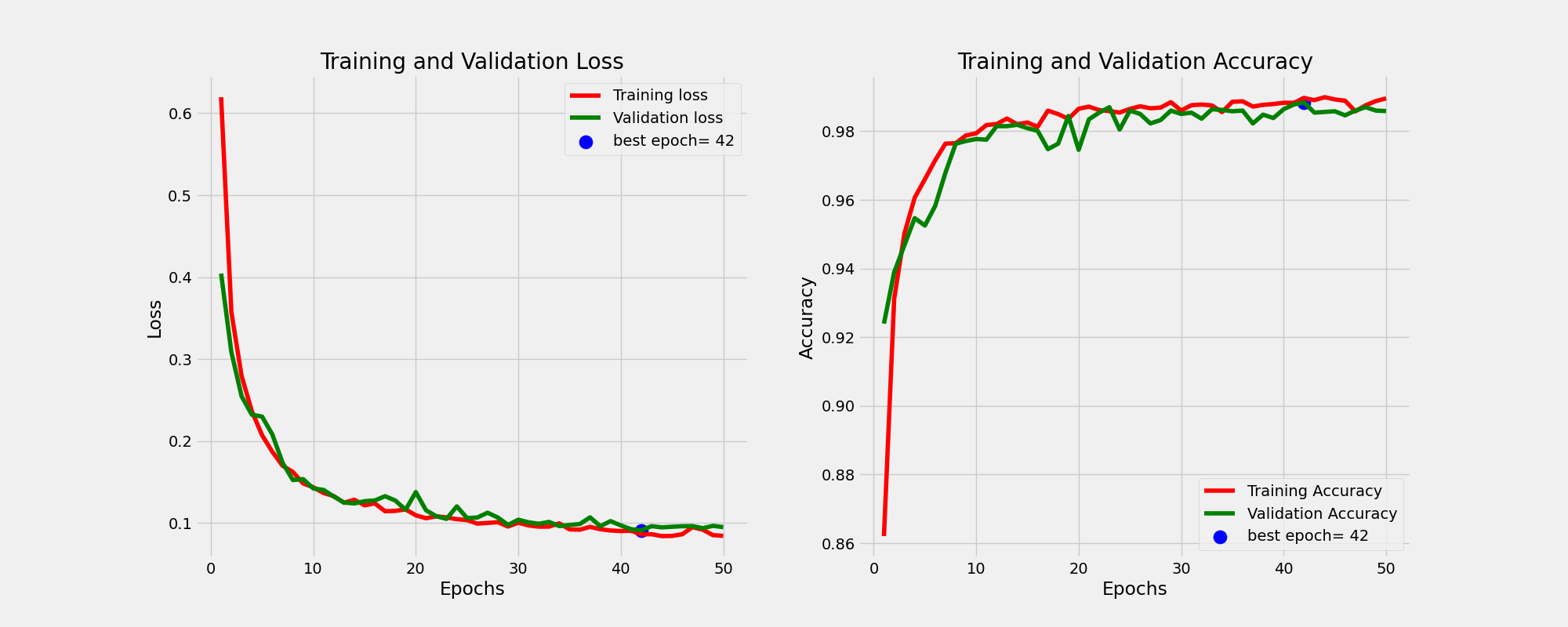
And this is the learning curves. For more information on how I perform the training please consult the train function of Classifier class in the utils.py script.
classification report
Test Loss: 0.118095263838768
Test Accuracy: 0.976578414440155
Predicting for 7856 samples
491/491 [==============================] - 10s 20ms/step
Classification Report:
              precision    recall  f1-score   support

      glioma       0.97      0.95      0.96      1797
  meningioma       0.96      0.96      0.96      1834
     notumor       1.00      1.00      1.00      2428
   pituitary       0.98      1.00      0.99      1797

    accuracy                           0.98      7856
   macro avg       0.98      0.97      0.97      7856
weighted avg       0.98      0.98      0.98      7856
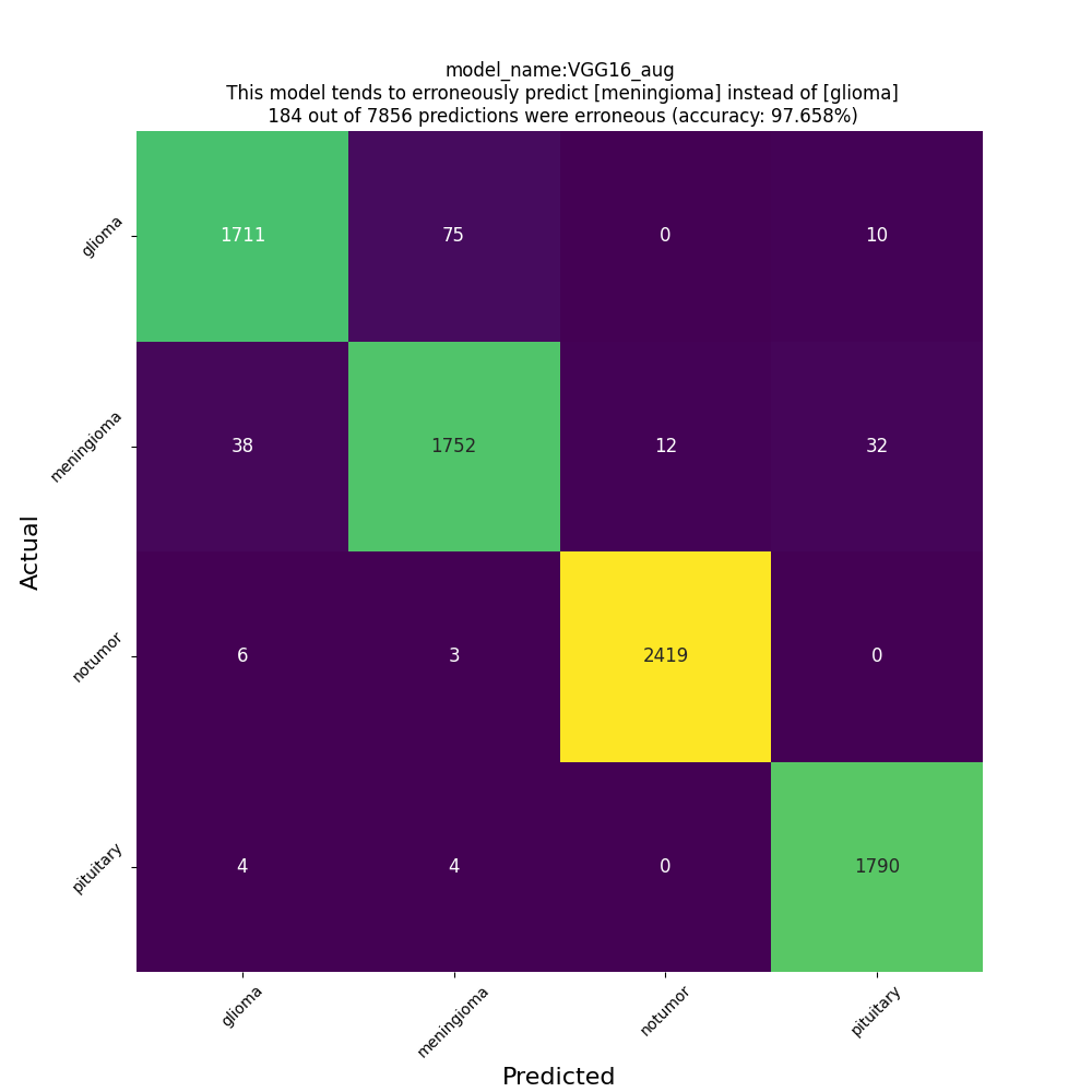
confusion matrix
VGG16 with the particular data augmentation seems to be promising even when we augment with slightly different way the test data. However, one should bear in mind that even the distribution of the test data of this particular MRI dataset taken from Kaggle is close enough to the distribution of the train data. This does not seem to be the case for images taken from the internet. My classifier, even the VGG16-based one, will most likely misclassify the unseen MRI images fetched from the internet. At this point I want to admit that due to lack of medical knowledge or expertise I am in no position to evaluate the quality of the training data themselves.
(brain)$ python3 src/diagnose_with_gui.py
