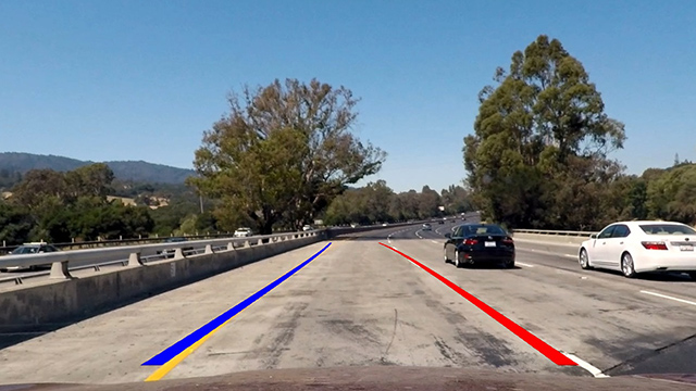
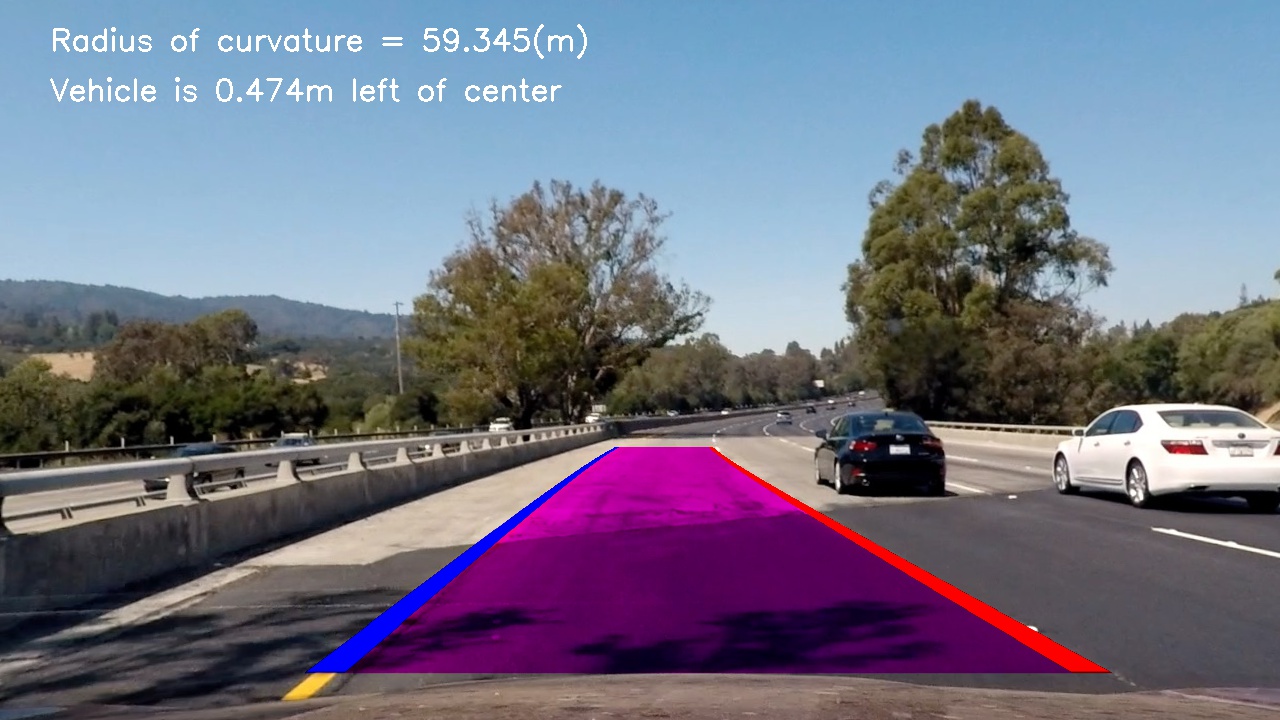
The goals / steps of this project are the following:
- Compute the camera calibration matrix and distortion coefficients given a set of chessboard images.
- Apply a distortion correction to raw images.
- Use color transforms, gradients, etc., to create a thresholded binary image.
- Apply a perspective transform to rectify binary image ("birds-eye view").
- Detect lane pixels and fit to find the lane boundary.
- Determine the curvature of the lane and vehicle position with respect to center.
- Warp the detected lane boundaries back onto the original image.
- Output visual display of the lane boundaries and numerical estimation of lane curvature and vehicle position.
Rubric Points
1. Briefly state how you computed the camera matrix and distortion coefficients. Provide an example of a distortion corrected calibration image.
The code for this step is found in camera_calibration.py. This script is near-boilerplate from Udacity. First, we log the objpoints and imgpoints identified with OpenCV's findChessboardCorners() function while looping through all the checkerboard images for calibration. Next we feed those values into the calibrateCamera() function and return our calibrated camera coordinates (mtx) and distortion coefficients (dist). Finally, we utilize undistort(), providing our newly-identified distortion information, to get the undistorted image seen below.
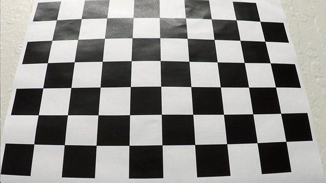
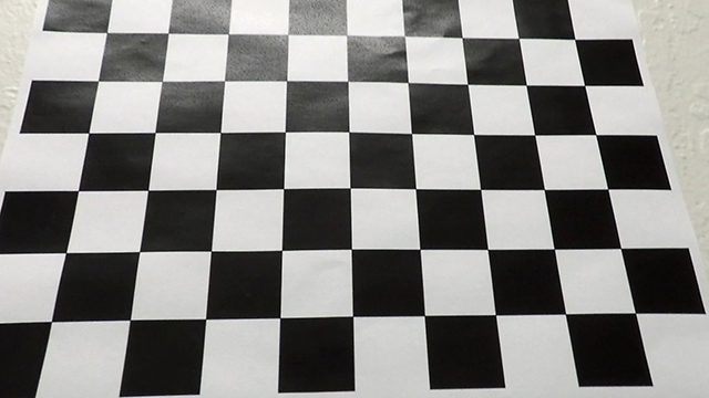
We saved my mtx and dist variables to the 'cal_pickle' file in our camera_calibration.py script. The same as in the prior step, we feed those values, along with our road images, to the undistort function. The result is shown below:
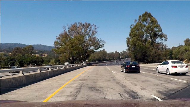
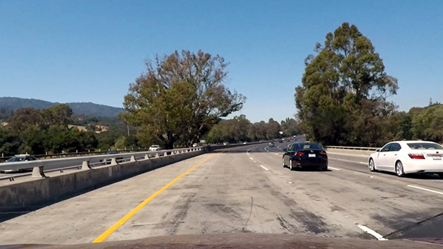
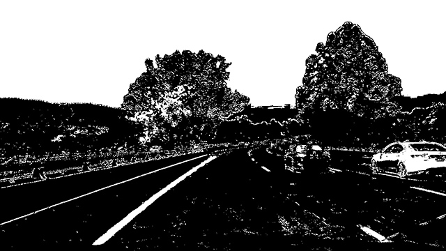
2. Describe how (and identify where in your code) you used color transforms, gradients or other methods to create a thresholded binary image. Provide an example of a binary image result.
We used the absolute value of the Sobel operator, as in the code from the Udacity lesson, to calculate the gradients of both the x and y directions of our image. It's the abs_sobel_thresh() function found at line 12 of our image_gen.py script. We also used the clever color_thresh() function (line 32) from the Udacity live training, first getting the threshold of the S channel of the HLS image and then the V channel of the converted HSV image to generate a binary image. See the example below:
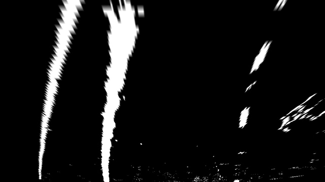
3. Describe how (and identify where in your code) you performed a perspective transform and provide an example of a transformed image.
Starting at line 103 in image_gen.py, we define a trapezoidal area in which my perspective transform should take place. We create both a 'src' and 'dst' matrix, and then feed those values to OpenCV's getPerspectiveTransform() function, logging it as M and grabbing its inverse for later to use on our final result. Here's an image to demonstrate the lane lines remain parallel:
4. Describe how (and identify where in your code) you identified lane-line pixels and fit their positions with a polynomial?
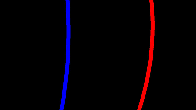
In tracker.py, primarily within the find_window_centroids() function at line 24, we use a sliding window method to find positive and negative gradient edges, and a convolution to squash those values into a histogram from which we can identify the valuable range of pixels.
Starting at line 117, to fit the line to the lanes, we create an array filled with the smoothed coordinates of the window-identified boxes via polyfit() line coordinates and feed it to the OpenCV fillPoly function.
5. Describe how (and identify where in your code) you calculated the radius of curvature of the lane and the position of the vehicle with respect to center.
We calculate the radius of curvature at line 153 of image_gen.py, converting from pixels to meters, using the following formula from this site:
R = (1 + (2*A*y + B)**2)**1.5 / max(1e-5, abs(2*A))
We calculate the offset at line 156, averaging the two points closest to the car to find the center and then scaling it by our pixels to meters multiplier (xm_per_pix).
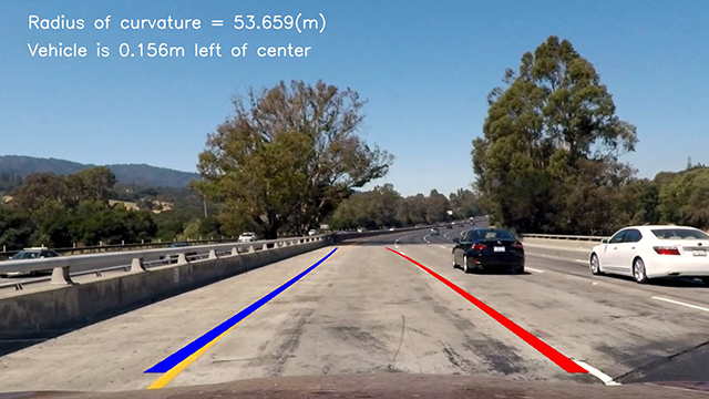
6. Provide an example image of your result plotted back down onto the road such that the lane area is identified clearly.
From lines 136-148, we use an additional set of lane lines to act as a mask for greater color depth of our lane markings and a center mask to create the colored patch between lane lines. From our Minv matrix, we use inverse perspective transform to return the new lane lines back to its original perspective, We use OpenCV.addweighted() to combine the original and masked lane line images.
1. Provide a link to your final video output. Your pipeline should perform reasonably well on the entire project video (wobbly lines are ok but no catastrophic failures that would cause the car to drive off the road!).
The video is created using the video_gen.py script, which is nearly identical to the pipeline detailed throughout this document. The essential difference is rather than exporting a series of images, it filters the video frame by frame and exports the result.
Here's a link to my video result
1. Briefly discuss any problems / issues you faced in your implementation of this project. Where will your pipeline likely fail? What could you do to make it more robust?
This project was a struggle. Though lots of the code was made available by Udacity, the process of working through all the different variables was very time-consuming. The live training was a big help, though it was hard after the fact to find values or my own methods that could really improve on those results. The pipeline could likely fail on extremely hard curves or in bright white or dark situations, or with a different color arrangement of asphalt and lane lines and has no concept of lane lines before or after to help compensate for brief or strange occurences in the visible lane lines. A revision of this project would work to take these factors into account through more robust color filtering and smoothing functions.
