Deep Cox proportional risk model and survival analysis implemented by tensorflow.
NOTE: tfdeepsurv-v2.0.0 has been released. The old version is on branch archive_v1. Compared with version v1.0, current version largely improved:
- speed on building computation graph
- utilizing raw tensorflow ops to compute loss function
- unified format of survival data
- code elegance and simplicity
DeepSurv, a package of Deep Cox proportional risk model, is open-source on Github. But our works may shine in:
- Supporting ties of death time in your survival data, which means different loss function and estimator of survival function (
Breslowapproximation). - Providing survival function estimation.
- Tuning hyperparameters of DNN using scientific method - Bayesian Hyperparameters Optimization.
- Implementing by the popular deep learning framework - tensorflow
Points needed to do in future version v2.1.0:
- requirements statement
- dockerfile and docker images of tfdeepsurv
- Github packge tools
Download TFDeepSurv package and install from the directory (Python version >= 3.5):
git clone https://github.com/liupei101/TFDeepSurv.git
cd TFDeepSurv
pip install .Read Notebook - tfdeepsurv_data_simulated.ipynb for more details!
from tfdeepsurv.datasets import load_simulated_data

### generate simulated data (Pandas.DataFrame)
# data configuration:
#     hazard ratio = 2000
#     number of features = 10
#     number of valid features = 2

# No. of training data = 2000
train_data = load_simulated_data(2000, N=2000, num_var=2, num_features=10, seed=1)
# No. of training data = 800
test_data = load_simulated_data(2000, N=800, num_var=2, num_features=10, seed=1)from tfdeepsurv.datasets import survival_stats
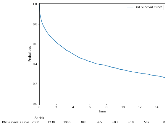
survival_stats(train_data, t_col="t", e_col="e", plot=True)result :
--------------- Survival Data Statistics ---------------
# Rows: 2000
# Columns: 10 + e + t
# Events Ratio: 0.74%
# Min Time: 0.0001404392
# Max Time: 15.0survival_stats(train_data, t_col="t", e_col="e", plot=False)
#--------------- Survival Data Statistics ---------------
# Rows: 2000
# Columns: 10 + e + t
# Events Ratio: 0.74%
# Min Time: 0.0001404392
# Max Time: 15.0The transformed survival data contains an new label. Negtive values are considered as right censored, and positive values are considered as event occurrence.
NOTE: In version 2.0, survival data must be transformed via tfdeepsurv.datasets.survival_df.
from tfdeepsurv.datasets import survival_df

surv_train = survival_df(train_data, t_col="t", e_col="e", label_col="Y")
surv_test = survival_df(test_data, t_col="t", e_col="e", label_col="Y")

# columns 't' and 'e' are packed into an new column 'Y'from tfdeepsurv import dsnn
input_nodes = 10
hidden_layers_nodes = [6, 3, 1]
# the arguments of dsnn can be obtained by Bayesian Hyperparameters Tuning
nn_config = {
"learning_rate": 0.7,
"learning_rate_decay": 1.0,
"activation": 'relu',
"L1_reg": 3.4e-5,
"L2_reg": 8.8e-5,
"optimizer": 'sgd',
"dropout_keep_prob": 1.0,
"seed": 1
}
# ESSENTIAL STEP: Pass arguments
model = dsnn(
input_nodes,
hidden_layers_nodes,
nn_config
)
# ESSENTIAL STEP: Build Computation Graph
model.build_graph()Y_col = ["Y"]
X_cols = [c for c in surv_train.columns if c not in Y_col]
# model saving and loading is also supported!
# read comments of `train()` function if necessary.
watch_list = model.train(
surv_train[X_cols], surv_train[Y_col],
num_steps=1900,
num_skip_steps=100,
plot=True
)result :
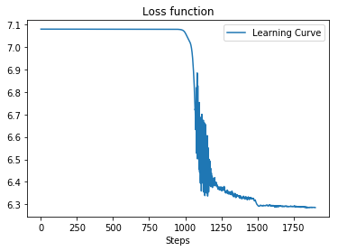
Average loss at step 100: 7.07983
Average loss at step 200: 7.07982
Average loss at step 300: 7.07981
...
Average loss at step 1700: 6.29165
Average loss at step 1800: 6.29007
Average loss at step 1900: 6.28687
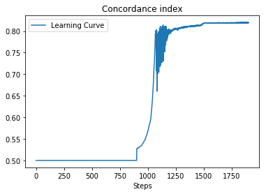
Curve of loss and CI:
| Loss Value | CI |
|---|---|
 |
 |
print("CI on training data:", model.evals(surv_train[X_cols], surv_train[Y_col]))
print("CI on test data:", model.evals(surv_test[X_cols], surv_test[Y_col]))
result :
CI on training data: 0.8193206851448683
CI on test data: 0.8175830825866967Model prediction includes:
- predicting hazard ratio or log hazard ratio
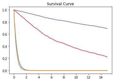
- predicting survival function
# predict log hazard ratio
print(model.predict(surv_test.loc[0:4, X_cols]))
# predict hazard ratio
print(model.predict(surv_test.loc[0:4, X_cols], output_margin=False))
result:
[[4.629786 ]
 [4.8222055]
 [0.       ]
 [1.4019105]
 [0.       ]]

[[102.49213 ]
 [124.2388  ]
 [  1.      ]
 [  4.062955]
 [  1.      ]]
# predict survival function
model.predict_survival_function(surv_test.loc[0:4, X_cols], plot=True)result:
The procedure on real-world data is similar with the described on simulated data. One we need to notice is data preparation.
More details can refer to Notebook - tfdeepsurv_data_real.ipynb.
We provide tools for hyperparameters tuning (Bayesian Hyperparameters Optimization) in deep neural network, which is automatic in searching optimal hyperparameters of DNN.
For more usage of Bayesian Hyperparameters Optimization, you can refer to here

