TensorGraph

TensorGraph is a framework for building any imaginable models based on TensorFlow.

As deep learning becomes more and more common and the architectures becoming more and more complicated, it seems that we need some easy to use framework to quickly build these models and that's what TensorGraph is designed for. It's a very simple and easy to use framework and allows you to build any imaginable models.

Target Audience

TensorGraph is targeted more at intermediate to advance users who feel keras or other packages is having too much restrictions on model building, and someone who don't want to rewrite the standard layers in tensorflow constantly, and someone who want to use some higher level layers to build models quickly without the restrictions of most other deep learning package.

Install

First you need to install tensorflow

To install tensorgraph simply do via pip

sudo pip install tensorgraph

or for bleeding edge version do

sudo pip install --upgrade git+https://github.com/hycis/TensorGraph.git@master

or simply clone and add to PYTHONPATH.

git clone https://github.com/hycis/TensorGraph.git
export PYTHONPATH=/path/to/TensorGraph:$PYTHONPATH

in order for the install to persist via export PYTHONPATH. Add PYTHONPATH=/path/to/TensorGraph:$PYTHONPATH to your .bashrc for linux or .bash_profile for mac. While this method works, you will have to ensure that all the dependencies in setup.py are installed.

How TensorGraph Works?

In TensorGraph, we defined three types of nodes

StartNode : for inputs to the graph
HiddenNode : for putting sequential layers inside
EndNode : for getting outputs from the model

We put all the sequential layers into a HiddenNode, and connect the hidden nodes together to build the architecture that you want. The graph always starts with StartNode and ends with EndNode. The StartNode is where you place your starting point, it can be a placeholder, a symbolic output from another graph, or data output from tfrecords. EndNode is where you want to get an output from the graph, where the output can be used to calculate loss or simply just a peek at the outputs at that particular layer. Below shows an example of building a tensor graph.

Graph Example

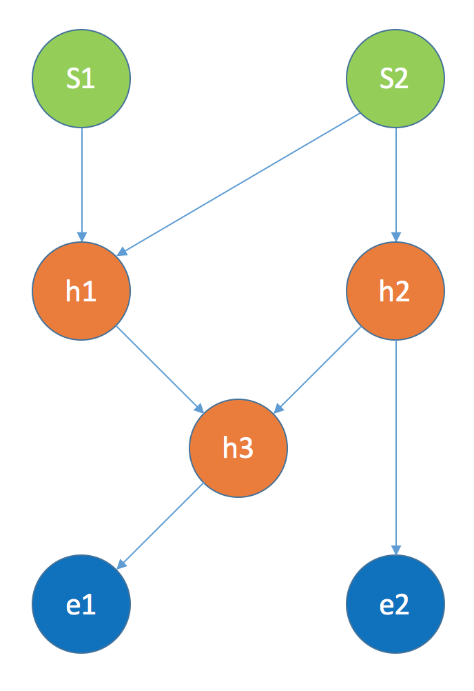
First define the StartNode for putting the input placeholder

y1_dim = 50
y2_dim = 100
batchsize = 32
learning_rate = 0.01

y1 = tf.placeholder('float32', [None, y1_dim])
y2 = tf.placeholder('float32', [None, y2_dim])
s1 = StartNode(input_vars=[y1])
s2 = StartNode(input_vars=[y2])

Then define the HiddenNode for putting the sequential layers in each HiddenNode

h1 = HiddenNode(prev=[s1, s2],
                input_merge_mode=Concat(),
                layers=[Linear(y1_dim+y2_dim, y2_dim), RELU()])
h2 = HiddenNode(prev=[s2],
                layers=[Linear(y2_dim, y2_dim), RELU()])
h3 = HiddenNode(prev=[h1, h2],
                input_merge_mode=Sum(),
                layers=[Linear(y2_dim, y1_dim), RELU()])

Then define the EndNode. EndNode is used to back-trace the graph to connect the nodes together.

e1 = EndNode(prev=[h3])
e2 = EndNode(prev=[h2])

Finally build the graph by putting StartNodes and EndNodes into Graph

graph = Graph(start=[s1, s2], end=[e1, e2])

Run train forward propagation to get symbolic output from train mode. The number of outputs from graph.train_fprop is the same as the number of EndNodes put into Graph

o1, o2 = graph.train_fprop()

Finally build an optimizer to optimize the objective function

o1_mse = tf.reduce_mean((y1 - o1)**2)
o2_mse = tf.reduce_mean((y2 - o2)**2)
mse = o1_mse + o2_mse
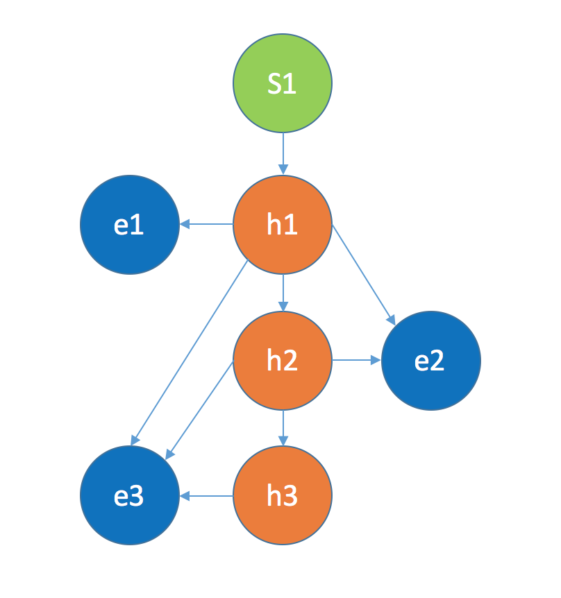
optimizer = tf.train.AdamOptimizer(learning_rate).minimize(mse)

Hierachical Softmax Example

Below is another example for building a more powerful hierachical softmax whereby the lower hierachical softmax layer can be conditioned on all the upper hierachical softmax layers.

## params
x_dim = 50
component_dim = 100
batchsize = 32
learning_rate = 0.01


x_ph = tf.placeholder('float32', [None, x_dim])
# the three hierachical level
y1_ph = tf.placeholder('float32', [None, component_dim])
y2_ph = tf.placeholder('float32', [None, component_dim])
y3_ph = tf.placeholder('float32', [None, component_dim])

# define the graph model structure
start = StartNode(input_vars=[x_ph])

h1 = HiddenNode(prev=[start], layers=[Linear(x_dim, component_dim), Softmax()])
h2 = HiddenNode(prev=[h1], layers=[Linear(component_dim, component_dim), Softmax()])
h3 = HiddenNode(prev=[h2], layers=[Linear(component_dim, component_dim), Softmax()])


e1 = EndNode(prev=[h1], input_merge_mode=Sum())
e2 = EndNode(prev=[h1, h2], input_merge_mode=Sum())
e3 = EndNode(prev=[h1, h2, h3], input_merge_mode=Sum())

graph = Graph(start=[start], end=[e1, e2, e3])

o1, o2, o3 = graph.train_fprop()

o1_mse = tf.reduce_mean((y1_ph - o1)**2)
o2_mse = tf.reduce_mean((y2_ph - o2)**2)
o3_mse = tf.reduce_mean((y3_ph - o3)**2)
mse = o1_mse + o2_mse + o3_mse
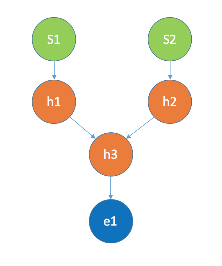
optimizer = tf.train.AdamOptimizer(learning_rate).minimize(mse)

Transfer Learning Example

Below is an example on transfer learning with bi-modality inputs and merge at the middle layer with shared representation, in fact, TensorGraph can be used to build any number of modalities for transfer learning.

## params
x1_dim = 50
x2_dim = 100
shared_dim = 200
y_dim = 100
batchsize = 32
learning_rate = 0.01


x1_ph = tf.placeholder('float32', [None, x1_dim])
x2_ph = tf.placeholder('float32', [None, x2_dim])
y_ph = tf.placeholder('float32', [None, y_dim])

# define the graph model structure
s1 = StartNode(input_vars=[x1_ph])
s2 = StartNode(input_vars=[x2_ph])

h1 = HiddenNode(prev=[s1], layers=[Linear(x1_dim, shared_dim), RELU()])
h2 = HiddenNode(prev=[s2], layers=[Linear(x2_dim, shared_dim), RELU()])
h3 = HiddenNode(prev=[h1,h2], input_merge_mode=Sum(),
                layers=[Linear(shared_dim, y_dim), Softmax()])

e1 = EndNode(prev=[h3])

graph = Graph(start=[s1, s2], end=[e1])
o1, = graph.train_fprop()

mse = tf.reduce_mean((y_ph - o1)**2)
optimizer = tf.train.AdamOptimizer(learning_rate).minimize(mse)