Supporting resources for System Dynamics Modeling with R
Welcome to the githib resource for the text book System Dynamics Modeling with R.
The text book is now available (in a number of formats) through the following links.
-
View on Springer System Dynamics Modeling with R
-
View on Amazon System Dynamics Modeling with R
With Springer's MyCopy, students and researchers can order their own personal, printed copy (or an eBook format) for 24.99 includes shipping and handling. This unique service is available to Institutions who have purchased one or more Springer eBook collections.
System Dynamics
System dynamics is a modeling methodology used to build simulation models of social systems, and these computerized models can support policy analysis and decision making. This simulation method is based calculus, and models of real-world dynamic processes are constructed using integral equations. The models presented here illustrate the breadth of application of system dynamics, and include:
- Epidemiology, with a focus on the contagious disease SIR model, and an interesting extension of this to a disaggregate form, based on a vectorized R implementation.
- Health Systems Design, which provides a system-wide model comprising population demographics, a supply chain of general practitioners, and a demand-capacity model of general practitioner services to overall population.
- Economics and Business, ranging from simple customer model, and onto models of limits to growth, capital investment, and the impact of non-renewable resources on growth.
Models are implemented using R and Vensim. The model catalog is as follows:
- Chapter 1 contains the Vensim model of customer growth, with a single stock (Customers), and two flows, an inflow (Recruits) and an outflow (Losses)
- Chapter 2 has an implemention of the customer model in R
- Chapter 3 presents models of (1) S-Shaped growth, (2) Solow's Economic model and (3) a model of overshoot and collapse.
- Chapter 4 introduces a Vensim model for a health systems example, where the model is divided into three distinct sectors
- Chapter 5 contains the SIR model and a vectorised diffusion model.
- Chapter 6 shows how RUnit can be used to test system dynamics models
- Chapter 7 illustrates how statistical screening can be used to analyse system dynamics models
R
R is open-source software (GNU General Public License), and has statistical, data manipulation, and visualization libraries. R is a functional programming language, where software programs are organized into functions that can be invoked to transform data. R is also object oriented. R’s mission is to enable the best and most thorough exploration of data possible (Chambers 2008). For this text, it is recommended to use the R Studio IDE, which is open source and provides an excellent way to manage R source files. Here is an example of a vector (similar to a one-dimensional array in languages such as C and Java), and how it can be manipulated. A key idea is know as vectorisation, where an operation (e.g. v*2) applied to a vector is applied to each vector element.
> v<-1:10
> v
 [1]  1  2  3  4  5  6  7  8  9 10
> v*2
 [1]  2  4  6  8 10 12 14 16 18 20
> v[1:3]
[1] 1 2 3
> max(v)
[1] 10
> min(v)
[1] 1
deSolve Package
For the system dynamics examples, the deSolve package is used. An example of a system dynamics model (the customer model) implemented using R and deSolve is shown below. These complete description of the code is contained in the text book, and comments are used here to provide an indication of how the model works.
library(deSolve)
library(ggplot2)
require(gridExtra)
library(scales)

# Setup simulation times and time step
START<-2015; FINISH<-2030; STEP<-0.25

# Create time vector
simtime <- seq(START, FINISH, by=STEP)

# Create stock and auxs
stocks  <- c(sCustomers=10000)
auxs    <- c(aGrowthFraction=0.08, aDeclineFraction=0.03)


# Model function
model <- function(time, stocks, auxs){
  with(as.list(c(stocks, auxs)),{

    fRecruits<-sCustomers*aGrowthFraction

    fLosses<-sCustomers*aDeclineFraction

    dC_dt <- fRecruits - fLosses

    return (list(c(dC_dt),
                 Recruits=fRecruits, Losses=fLosses,
                 GF=aGrowthFraction,DF=aDeclineFraction))
  })
}


# Run simulation
o<-data.frame(ode(y=stocks, times=simtime, func = model,
                  parms=auxs, method="euler"))
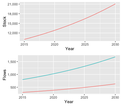
R's ggplot2 package is then used to visualize the simulation output (which is held in a data frame.)
p1<-ggplot()+
  geom_line(data=o,aes(time,o$sCustomers,color="Customers"))+
  scale_y_continuous(labels = comma)+
  ylab("Stock")+
  xlab("Year") +
  labs(color="")+
  theme(legend.position="none")


p2<-ggplot()+
  geom_line(data=o,aes(time,o$Losses,color="Losses"))+
  geom_line(data=o,aes(time,o$Recruits,color="Recruits"))+
  scale_y_continuous(labels = comma)+
  ylab("Flows")+
  xlab("Year") +
  labs(color="")+
  theme(legend.position="none")

p3<-grid.arrange(p1, p2,nrow=2, ncol=1)
The output aligns the two plots, with the flows together on the lower plot, and the stock on the upper plot. As the inflow (0.08) exceeds the outflow (0.03), the stock rises (exponentially).
System Dynamics Simulation Tools
The following are useful links to system dynamics software, which can be used to build system dynamics models.

