Pymc3-based universal time series prediction and decomposition library (inspired by Facebook Prophet). However, while Faceook prophet is a well-defined model, pm-prophet allows for total flexibility in the choice of priors and thus is potentially suited for a wider class of estimation problems
To install:
pip install pmprophet
What's implemented:
- Nowcasting & Forecasting
- Intercept, growth
- Regressors
- Holidays
- Additive & multiplicative seasonality
- Fitting and plotting
- Custom choice of priors (not included in the original prophet)
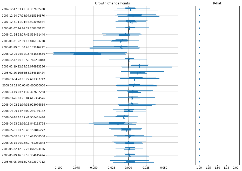
- Changepoints in growth
- Fitting with NUTS/AVDI/Metropolis
Differencies with respect to Facebook Prophet:
- Saturating growth is not implemented
- Uncertainty estimation is different
- All components (including seasonality) need to be explicitly added to the model
- By design pm-prophet places a big emphasis on posteriors and uncertainty estimates, and therefore it won't use MAP for it's estimates.
- While Faceook prophet is a well-defined fixed model, pm-prophet allows for total flexibility in the choice of priors and thus is potentially suited for a wider class of estimation problems
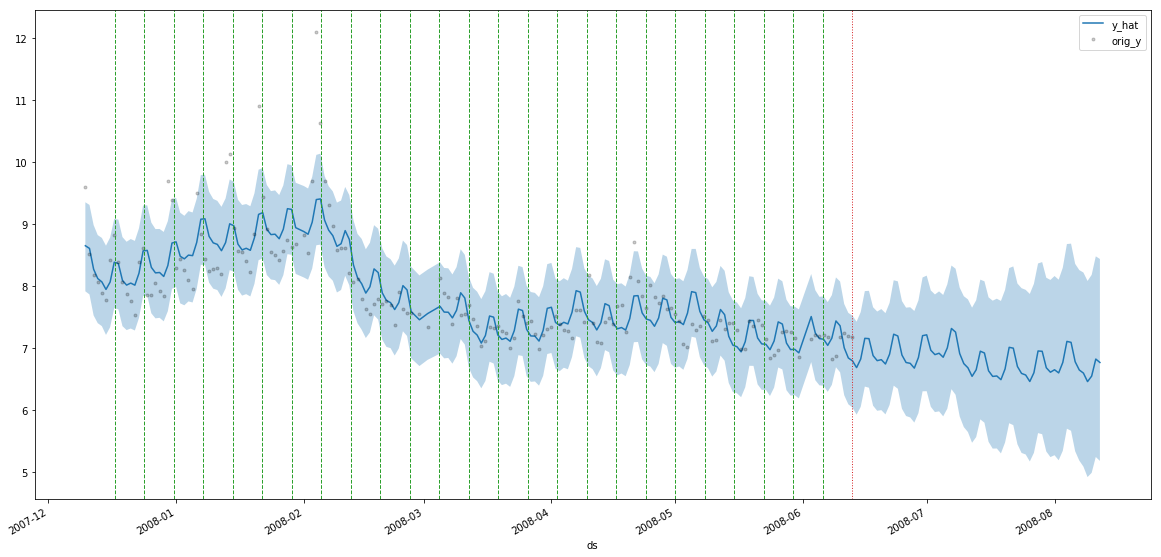
Predicting the Peyton Manning timeseries:
import pandas as pd
from pmprophet.model import PMProphet
df = pd.read_csv("/Users/luca/pm-prophet/examples/example_wp_log_peyton_manning.csv")
df = df.head(180)
# Fit both growth and intercept
m = PMProphet(df, growth=True, intercept=True, n_changepoints=25, changepoints_prior_scale=.01, name='model')
# Add monthly seasonality (order: 3)
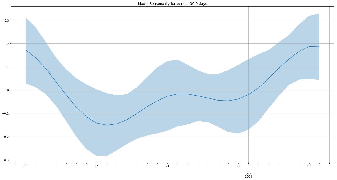
m.add_seasonality(seasonality=30, fourier_order=3)
# Add weekly seasonality (order: 3)
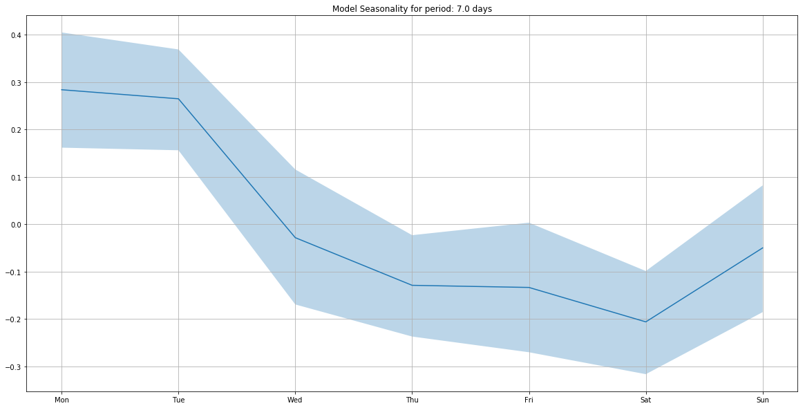
m.add_seasonality(seasonality=7, fourier_order=3)
# Fit the model (using NUTS)
m.fit(method='NUTS')
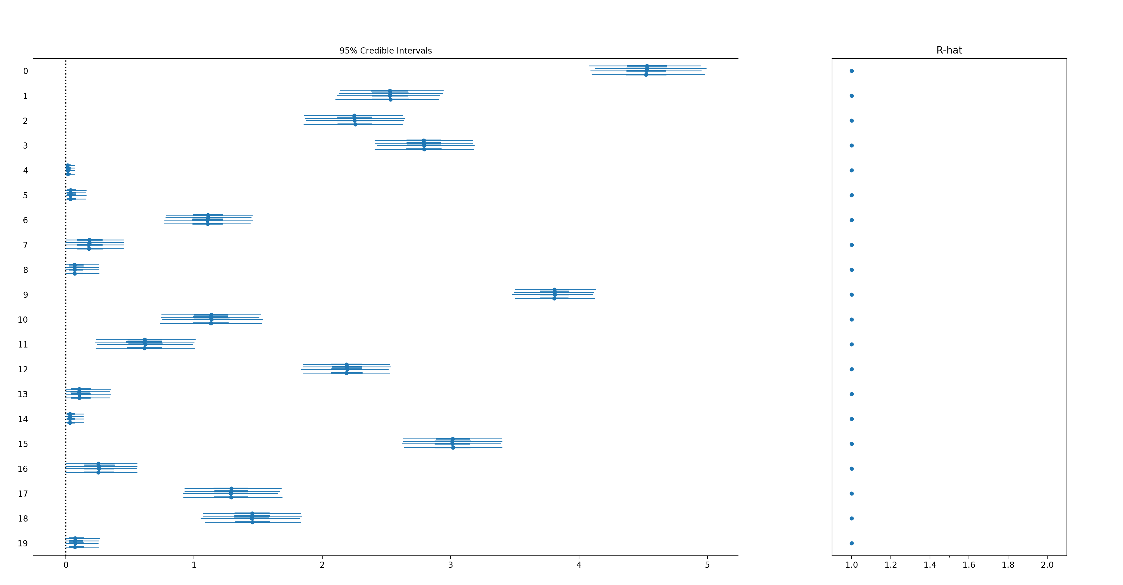
ddf = m.predict(60, alpha=0.2, include_history=True, plot=True)
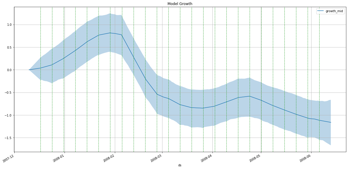
m.plot_components(
intercept=False,
)
One of the main reason why PMProphet was built is to allow custom priors for the modeling.
The default priors are:
| Variable | Prior | Parameters |
|---|---|---|
regressors |
Normal | loc:0, scale:10 |
holidays |
Laplace | loc:0, scale:10 |
seasonality |
Laplace | loc:0, scale:0.05 |
growth |
Laplace | loc:0, scale:10 |
changepoints |
Laplace | loc:0, scale:10 |
intercept |
Normal | loc:y.mean, scale: 2 * y.std |
sigma |
Half Cauchy | loc:100 |
But you can change model priors by inspecting and modifying the distribution in
m.priorswhich is a dictionary of {prior: pymc3-distribution}.
In the example below we will model an additive time-series by imposing a "positive coefficients" constraint by using an Exponential distribution instead of a Laplacian distribution for the regressors.
import pandas as pd
import numpy as np
import pymc3 as pm

n_timesteps = 100
n_regressors = 20

regressors = np.random.normal(size=(n_timesteps, n_regressors))
coeffs = np.random.exponential(size=n_regressors) + np.random.normal(size=n_regressors)
# Note that min(coeffs) could be negative due to the white noise

regressors_names = [str(i) for i in range(n_regressors)]

df = pd.DataFrame()
df['y'] = np.dot(regressors, coeffs)
df['ds'] = pd.date_range('2017-01-01', periods=n_timesteps)
for idx, regressor in enumerate(regressors_names):
    df[regressor] = regressors[:, idx]

m = PMProphet(df, growth=False, intercept=False, n_changepoints=0, name='model')

with m.model:
    # Remember to suffix _<model-name> to the custom priors
    m.priors['regressors'] = pm.Exponential('regressors_%s' % m.name, 1, shape=n_regressors)

for regressor in regressors_names:
    m.add_regressor(regressor)

m.fit(
    draws=10 ** 4,
    method='NUTS',
)
m.plot_components()