Welcome to the repository for the "Energy-Based Analog Neural Network Framework" presented in the 2022 edition of the IEEE SOCC conference. The associated paper can be accessed on ieee explore or downloaded from this link.
This repository contains the code for the framework and is currently undergoing development. In the future, we plan to provide additional examples to further showcase the capabilities and versatility of the framework. We appreciate your interest in our work and hope that the provided code is of use to you."
EBANA (Energy-Based Analog Neural Network Framework) is a deep learning framework designed to train analog neural networks using the Equilibrium Propagation algorithm. Inspired by the simplicity and flexibility of Keras, EBANA aims to make machine learning and analog electronics accessible to a wider audience by providing an easy-to-use and intuitive API. With EBANA, users can easily experiment with different network architectures and evaluate the tradeoffs that exist in the design space.
For more information on the Equilibrium Propagation algorithm, please see this paper: https://arxiv.org/abs/1602.05179"
EBANA leverages the power of Ngspice for SPICE simulation and utilizes PySpice to provide seamless interoperability between Python and Ngspice.
Assuming you already have conda
installed (for example, through
miniconda), the required
packages can be installed using the code below:
conda create -n ebana
conda activate ebana
conda install -c conda-forge pyspice
conda install -c conda-forge ngspice ngspice-lib
The next step is to make a clone of this repository:
git clone https://github.com/mawatfa/ebana.gitThe easiest way to try out the ebana framework is through Docker. This allows you to quickly set up the necessary environment and dependencies, so you can start experimenting with the framework right away.
To set up the ebana framework using docker, follow these steps:
-
Open a terminal and
cdto thedocker-setupdirectory. -
Run the command
docker build -t ebana .. This will build an image with the nameebanabased on the instructions in thedockerfile. This process may take a few minutes to complete. -
Once the image has been created, you can create a container by running
docker run -it --name ebana_container ebana. -
If you need to reattach to the container after it has exited, use the commands
docker container start ebana_containeranddocker attach ebana_container.
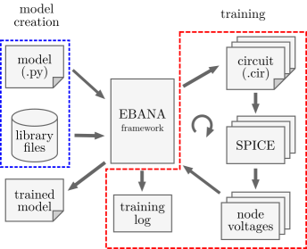
The EBANA framework is largely made up of two parts: one for defining the network model, and the other for training in the analog domain. A block diagram of the framework is shown below.
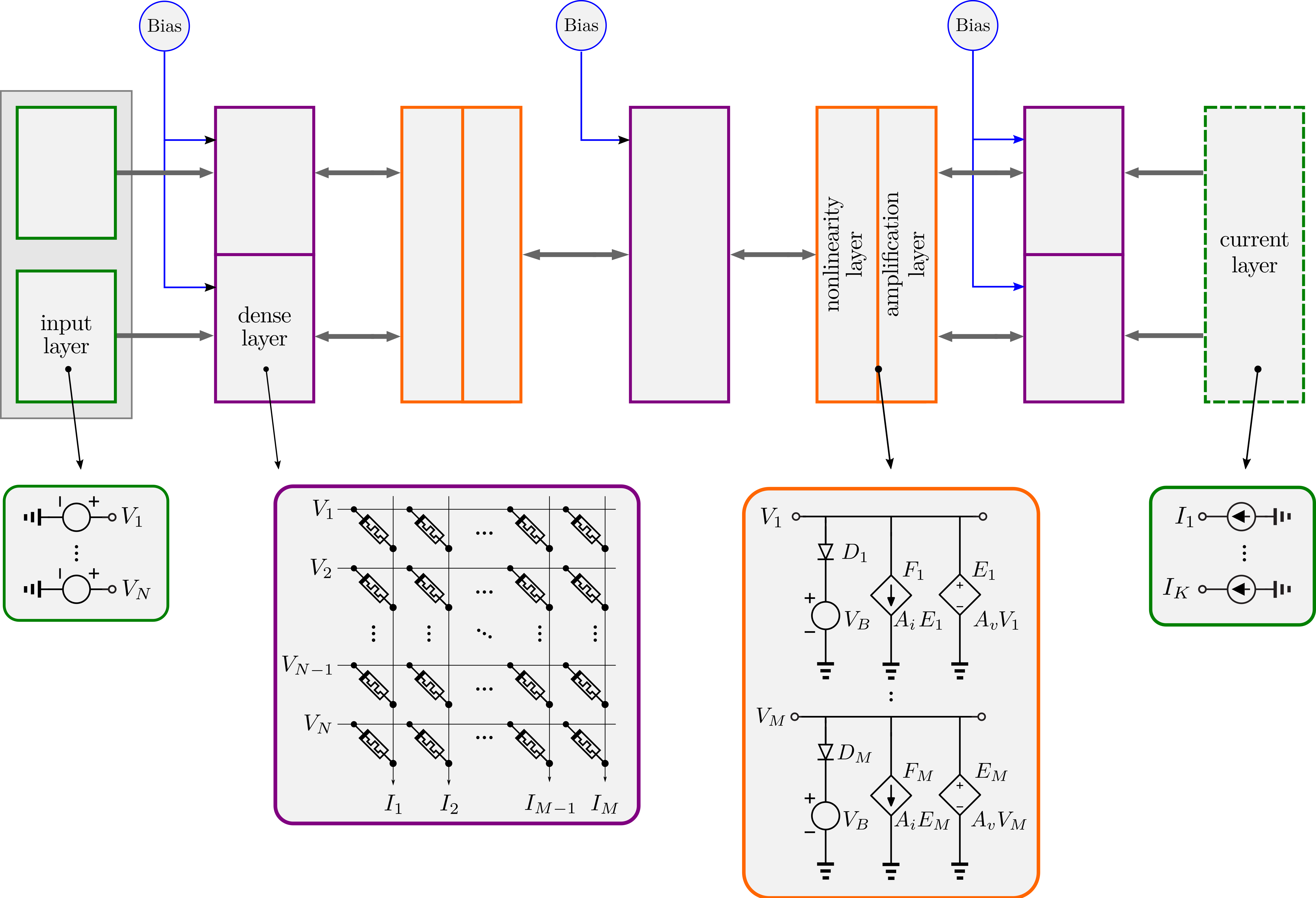
The process of designing and training a model in EBANA starts with defining the model. The general structure of an analog neural network that can be trained with EBANA is shown below. It consists of an input layer, several hidden layers, and an output layer. It looks similar to a regular neural network that can be trained by the backpropagation algorithm except for two major differences. First, the layers can influence each other bidirectionally. Second, the output nodes are linked to current sources which serve to inject loss gradient signals during training
An example of a topology that can be used to learn the xor dataset
is given below. The complete example for the xor training along with others
can found in the test_circuit directory.
Constructing a neural network topology in EBANA follows the Keras syntax very closely.
# input layer
xp  = InputVoltageLayer(units=input_units, name='xp')
xn = InputVoltageLayer(units=input_units, name='xn')
b1_p = BiasVoltageLayer(units=1, name='b1_p', bias_voltage=bias_p)
b1_n = BiasVoltageLayer(units=1, name='b1_n', bias_voltage=bias_n)
j1 = ConcatenateLayer(name='j1')([xp, xn, b1_p, b1_n])

# hidden dense layer 1
d1 = DenseLayer(units=hidden_1_units, lr=4e-8, name='d1', initializer=weight_initialzier, trainable=True)(j1)
a1_1 = DiodeLayer(name='act1_1', direction='down', bias_voltage=down_diode_bias, trainable=False, kind="behavioral", param=behaviorial_diode_param)(d1)
a1_2 = DiodeLayer(name='act1_2', direction='up', bias_voltage=up_diode_bias, trainable=False, kind="behavioral", param=behaviorial_diode_param)(a1_1)
g1 = AmplificationLayer(name='amp1', param=amp_param)(d1)

# layer before last
b2_p = BiasVoltageLayer(units=1, name='b2_p', bias_voltage=bias_p)
b2_n = BiasVoltageLayer(units=1, name='b2_n', bias_voltage=bias_n)
j2 = ConcatenateLayer(name='j2')([g1, b2_p, b2_n])

# output layer
d_out = DenseLayer(units=2 * output_units, lr=4e-8, name='d_out', initializer=weight_initialzier, trainable=True)(j2)
c_out = CurrentLayer(name='xor')(d_out)

model = Model(inputs=[xp, xn, b1_p, b2_p, b1_n, b2_n], outputs=[c_out])
The network defined in the example above consists of four blocks:
-
The input block is where the inputs to the model are provided. In this case, there are four input sources:
xp,xn,b1_p, andb1_n.- The
xordataset typically only has a single input source, represented byxp. - However, in analog circuits, negative weights are represented by
resistors with a positive value, so a second set of inputs with opposite
polarity is added, represented by
xn. - It is also common in analog neural networks to set the bias to values
other than 1, which is why there are input sources
b1_pandb1_n. - These four input sources are concatenated and passed to the next layer."
- The
-
The second block is the first hidden layer, consisting of a dense layer, two nonlinearity layers, and an amplification layer.
- The syntax for the dense layer is similar to that of Keras, with the added ability to define a custom learning rate for each layer.
- The nonlinearity is implemented using two diode layers, which can be
customized using the parameters
bias_voltage,direction,model, anduse_mos. - In analog circuits, it is important to maintain the signal amplitude as it
passes through the components, which can be achieved using the
amplification layer with a customizable
gainparameter."
-
The third block simply takes the output from the previous layer, adds a custom bias to it, and passes the result to the next layer.
-
The last block is the output block, which is represented by a dense layer. This layer is defined in a similar manner to the dense layer in the hidden layer, with the exception that the number of output nodes is doubled to account for negative weights. Additionally, a layer of current sources is attached to the output node in order to inject current into the circuit during the second phase of training. This injected current serves as the loss gradient in the backpropagation algorithm.
Training the model is almost exactly the same as in Keras. An example is shown below.
save_name = "xor2_test"

optimizer = optimizers.Adam(model, beta=beta)
#optimizer.load_state(f"{save_name}_optimizer.pickle")

metrics = metrics.Metrics(
    model,
    # save_output_voltages="last",
    # save_power_params="last",
    verbose = True,
    validate_every={"epoch_num": 10},
)

loss_fn = losses.MSE(output_midpoint=output_midpoint)

model.fit(
    train_dataloader=train_dataloader,
    beta=beta,
    epochs=100,
    loss_fn=loss_fn,
    optimizer=optimizer,
    test_dataloader=test_dataloader,
    metrics=metrics,
)

predictions = model.evaluate(train_dataset, loss_fn=loss_fn)
Three things must be specified in order to train the model:
- The optimizer: at this stage, it is possible to load the optimizer state from a previous run if you want to resume training or reuse some trained layers.
- Metrics for tracking loss and accuracy during simulation, saving voltages and power parameters, etc.
- The loss function, such as mean squared error (MSE), binary cross entropy (BCE), or cross entropy (CrossEntropyLoss).
- The fit method: This includes the specification of dataloaders for the training and test datasets, the optimizer, loss function, number of epochs, and the frequency at which the model should be validated against the test dataset (e.g. after every n batches or epochs of training).
Having trained the model, it is possible to save the weights, optimizer states, loss history, test dataset accuracy, etc. This is done using the code below.
optimizer.save_state(save_name + "_optimizer.pickle")
model.save_history(save_name + "_history.pickle")New analog blocks can be easily created using PySpice. A short tutorial on the usage of PySpice can be found here.

