import BeamProp_Script as bs      # This is the script that handles the propagation
import sympy as sym               # For Symbolic examples
import numpy as np                # Handling of lists and for plotting
import matplotlib.pyplot as plt # Plottinghelp(bs)Help on module BeamProp_Script:
NAME
BeamProp_Script - Created on Wed Feb 19 15:51:54 2020
DESCRIPTION
@author: wrighta
FUNCTIONS
W0(zr, lam)
Parameters
----------
zr : float, integer, symbol
Rayleigh range in meters
lam : float, integer, symbol
Wavelength of light in meters
Returns
-------
w0 : float, integer, symbol
Beam waist radius in meters
Zr(wo, lam)
Parameters
----------
wo : float, integer, or symbol
Beam waist radius in meters.
lam : float, integer, or symbol
Wavelength of light in meters.
Returns
-------
zr : float, int, symbols
Rayleigh range for given beam waist and wavelength.
lens(f)
Parameters
----------
f : float or integer or sympy symbol in meters
Thin lens focal length in meters
Returns
-------
mat : 2x2 matrix
[
[ 1, 0],
[-1/f, 1]
]
mult(mat1, *argv)
Parameters
----------
mat1 : 2x2 ABCD matrix
Last matrix light interacts with.
*argv : 2x2 ABCD matrices
From left to right, the matrices should be entered such that the leftmost matrix interacts
with light temporally after the rightmost matrix.
Returns
-------
Mat : 2x2 matrix
The ABCd matrix describing the whole optical system.
plot(func, var, rang=array([0. , 0.01, 0.02, 0.03, 0.04, 0.05, 0.06, 0.07, 0.08, 0.09, 0.1 ,
0.11, 0.12, 0.13, 0.14, 0.15, 0.16, 0.17, 0.18, 0.19, 0.2 , 0.21,
0.22, 0.23, 0.24, 0.25, 0.26, 0.27, 0.28, 0.29, 0.3 , 0.31, 0.32,
0.33, 0.34, 0.35, 0.36, 0.37, 0.38, 0.39, 0.4 , 0.41, 0.42, 0.43,
0.44, 0.45, 0.46, 0.47, 0.48, 0.49, 0.5 , 0.51, 0.52, 0.53, 0.54,
0.55, 0.56, 0.57, 0.58, 0.59, 0.6 , 0.61, 0.62, 0.63, 0.64, 0.65,
0.66, 0.67, 0.68, 0.69, 0.7 , 0.71, 0.72, 0.73, 0.74, 0.75, 0.76,
0.77, 0.78, 0.79, 0.8 , 0.81, 0.82, 0.83, 0.84, 0.85, 0.86, 0.87,
0.88, 0.89, 0.9 , 0.91, 0.92, 0.93, 0.94, 0.95, 0.96, 0.97, 0.98,
0.99, 1. , 1.01, 1.02, 1.03, 1.04, 1.05, 1.06, 1.07, 1.08, 1.09,
1.1 , 1.11, 1.12, 1.13, 1.14, 1.15, 1.16, 1.17, 1.18, 1.19, 1.2 ,
1.21, 1.22, 1.23, 1.24, 1.25, 1.26, 1.27, 1.28, 1.29, 1.3 , 1.31,
1.32, 1.33, 1.34, 1.35, 1.36, 1.37, 1.38, 1.39, 1.4 , 1.41, 1.42,
1.43, 1.44, 1.45, 1.46, 1.47, 1.48, 1.49, 1.5 , 1.51, 1.52, 1.53,
1.54, 1.55, 1.56, 1.57, 1.58, 1.59, 1.6 , 1.61, 1.62, 1.63, 1.64,
1.65, 1.66, 1.67, 1.68, 1.69, 1.7 , 1.71, 1.72, 1.73, 1.74, 1.75,
1.76, 1.77, 1.78, 1.79, 1.8 , 1.81, 1.82, 1.83, 1.84, 1.85, 1.86,
1.87, 1.88, 1.89, 1.9 , 1.91, 1.92, 1.93, 1.94, 1.95, 1.96, 1.97,
1.98, 1.99, 2. , 2.01, 2.02, 2.03, 2.04, 2.05, 2.06, 2.07, 2.08,
2.09, 2.1 , 2.11, 2.12, 2.13, 2.14, 2.15, 2.16, 2.17, 2.18, 2.19,
2.2 , 2.21, 2.22, 2.23, 2.24, 2.25, 2.26, 2.27, 2.28, 2.29, 2.3 ,
2.31, 2.32, 2.33, 2.34, 2.35, 2.36, 2.37, 2.38, 2.39, 2.4 , 2.41,
2.42, 2.43, 2.44, 2.45, 2.46, 2.47, 2.48, 2.49, 2.5 , 2.51, 2.52,
2.53, 2.54, 2.55, 2.56, 2.57, 2.58, 2.59, 2.6 , 2.61, 2.62, 2.63,
2.64, 2.65, 2.66, 2.67, 2.68, 2.69, 2.7 , 2.71, 2.72, 2.73, 2.74,
2.75, 2.76, 2.77, 2.78, 2.79, 2.8 , 2.81, 2.82, 2.83, 2.84, 2.85,
2.86, 2.87, 2.88, 2.89, 2.9 , 2.91, 2.92, 2.93, 2.94, 2.95, 2.96,
2.97, 2.98, 2.99]))
Parameters
----------
func : Sympy function of one variable
Sympy function defining the beam width after the last optical element.
var : sympy variable
Variable in func that will be plotted.
rang : numpy array
Array of the values along the optical axis to be plotted
Returns
-------
plot : matplotlib graph
Graph of the beam width of var
prop(d)
Parameters
----------
d : float or integer or sympy symbol
Distance light is propagating along the z-axis.
Returns
-------
mat: 2x2 matrix
[
[1, d],
[0, 1]
]
q1_func(z, w0, lam, mat)
Parameters
----------
z : float, int, symbol
Position of the beam waist in meters.
w0 : float, int, symbol
Radial waist size in meters (of the embedded Gaussian, i.e. W0/M).
lam : float, int, symbol
Wavelength of light in meters.
mat : float, int, symbol
The ABCD 2x2 matrix describing the optical system.
Returns
-------
z: float, int, symbol
Position of the beam waist after the optical system
zr: float, int, symbol
Rayleigh range of the beam after the optical system
q1_inv_func(z, w0, lam, mat)
Parameters
----------
z : float, int, symbol
Position of the beam waist in meters.
w0 : float, int, symbol
Radial waist size in meters (of the embedded Gaussian, i.e. W0/M).
lam : float, int, symbol
Wavelength of light in meters.
mat : float, int, symbol
The ABCD 2x2 matrix describing the optical system.
Returns
-------
R : float, int, symbol
Radius of curvature of the wavefront in meters.
w : float, int, symbol
Radius of the beam in meters.
ray(y, theta)
Parameters
----------
y : float or integer or sympy symbol in meters
The vertical height of a ray.
theta : float or integer in radians
The angle of divergence of the ray.
Returns
-------
mat : 2x1 matrix
[
[y],
[teta]
]
DATA
oo = oo
FILE
c:\users\wrighta\documents\beamprop\beamprop_script.py
A Gaussian beam can be defined by it's (radial) waist, $w_0$ , it's Rayleigh range, $z_R = \frac{\pi * w_0^2}{\lambda}$ , and the location of its waist, $z_0$ .
w0 = 1E-3 # 1mm beam waist
lam = 355E-9 # wavelength of 355 nm (UV)
zR = bs.Zr(w0, lam) # Rayleigh range in m
z0 = 0 # location of waist in m
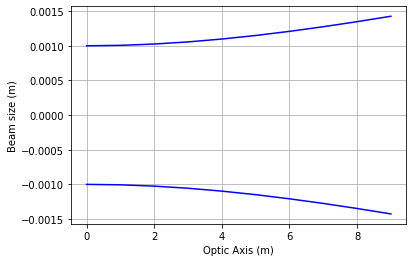
We now want to define our "optical system" using matrices. For this first example, we will just use a free space propagation matrix, and let the beam propagate a distance $d$ which we will define using a symbol.
d = sym.symbols('d')
M = bs.prop(d)
We now use the bs script to do all the ABCD and q-parameter math, and return the waist and radius of curvature functions
R, w = bs.q1_inv_func(0, w0, lam, M)print('w = {}'.format(w))w = 0.001*(0.0127690021685256*d**2 + 1)**0.5
bs.plot(w, d, rang = np.arange(0,10))Let's show what happens when a beam travels through a lens. We use the "mult" function to multiply multiple ABCD matrices together.
w0 = 1E-3 # 1mm beam waist
lam = 355E-9 # wavelength of 355 nm (UV)
zR = bs.Zr(w0, lam) # Rayleigh range in m
z0 = 0 # location of waist in m

d = sym.symbols('d')
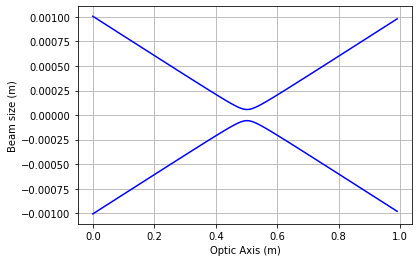
M = bs.mult(bs.prop(d), bs.lens(.5), bs.prop(1))

R, w = bs.q1_inv_func(0, w0, lam, M)

bs.plot(w, d, rang = np.arange(0,1,.01))w0 = 1E-3 # 1mm beam waist
lam = 355E-9 # wavelength of 355 nm (UV)
zR = bs.Zr(w0, lam) # Rayleigh range in m
z0 = 0 # location of waist in m
d1, d2, d3, f1, f2 = sym.symbols('d1 d2 d3 f1 f2')
M = bs.mult(bs.prop(d3),bs.lens(f2),bs.prop(d2), bs.lens(f1), bs.prop(d1))
R, w = bs.q1_inv_func(0, w0, lam, M)For example, lets say the beam travels 1 m before hitting the first lens, and we want the beam to be 5x w0 after coming out of the second lens. We substitute d1 for 1 meter, since the beam propagates 1 meter, and we substitute d3 for 0, since we only care about the beam size right at the second lens. This gives us a relation between f1 and d2 (the separation between the lenses).
w = w.subs(d1,1).subs(d3,0)
f1_eq = sym.solve(w - 5*w0, f1)[0]
print('f = {}'.format(f1_eq))
f = 1.0084642216545e+15*d2*(1.12051580183833e+27*d2 - 4.41556446152598e+29*sqrt(1 - 0.000504320418227052*d2**2) + 8.88733242867719e+28)/(1.13000009595246e+42*d2**2 + 2.26000019190491e+42*d2 - 2.12276362486616e+45)
print('f1 = {:.2f} m, for a lens separation of 1 meter'.format(f1_eq.subs(d2, 1)))f1 = 0.17 m, for a lens separation of 1 meter
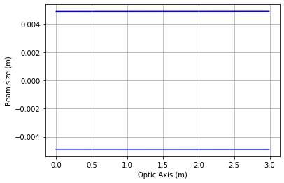
There are a couple different ways to think about collimation. One is that the beam size doesn't change over a long distance. The other is that the radius of curvature is infinite (i.e. a plane wave). Lets us the latter interpretation. Thus, we want to find the focal length f2 that makes R infinite, or that makes 1/R =0.
R_coll = R.subs(d1,1).subs(d2,1).subs(f1,.17).subs(d3,0)
f2_coll = sym.solve(1/R_coll,f2)[0]
print('f2 = {:.2f}, for a collimated beam, 5x the original waist, after propagating 1m to the first lens of f1 = .17m, and propagating another 1m to the second lens'.format(f2_coll))
f2 = 0.83, for a collimated beam, 5x the original waist, after propagating 1m to the first lens of f1 = .17m, and propagating another 1m to the second lens
M = bs.mult(bs.prop(d3),bs.lens(.83),bs.prop(1), bs.lens(.17), bs.prop(1))

R, w = bs.q1_inv_func(0, w0, lam, M)

bs.plot(w,d3)expansion_factor = w.subs(d3,0)/ w0
print('beam is w = {:.2f} x w0'.format(expansion_factor))beam is w = 4.90 x w0
beam_size_change = (w.subs(d3,10) - w.subs(d3,0)) / w.subs(d3,0) * 100
print('Over 10 m after second lens, beam changes by {:.0f}%'.format(beam_size_change))
Over 10 m after second lens, beam changes by 1%


