scipy_dae - solving differential algebraic equations (DAE's) and implicit differential equations (IDE's) in Python

Python implementation of solvers for differential algebraic equations (DAE's) and implicit differential equations (IDE's) that should be added to scipy one day.

Currently, two different methods are implemented.

Implicit Radau IIA methods of order 2s - 1 with arbitrary number of odd stages.
Implicit backward differentiation formula (BDF) of variable order with quasi-constant step-size and stability/ accuracy enhancement using numerical differentiation formula (NDF).

More information about both methods are given in the specific class documentation.

To pique your curiosity

The Kármán vortex street solved by a finite element discretization of the weak form of the incompressible Navier-Stokes equations using FEniCS and the three stage Radau IIA method.

Basic usage

The Robertson problem of semi-stable chemical reaction is a simple system of differential algebraic equations of index 1. It demonstrates the basic usage of the package.

import numpy as np
import matplotlib.pyplot as plt
from scipy_dae.integrate import solve_dae


def F(t, y, yp):
    """Define implicit system of differential algebraic equations."""
    y1, y2, y3 = y
    y1p, y2p, y3p = yp

    F = np.zeros(3, dtype=np.common_type(y, yp))
    F[0] = y1p - (-0.04 * y1 + 1e4 * y2 * y3)
    F[1] = y2p - (0.04 * y1 - 1e4 * y2 * y3 - 3e7 * y2**2)
    F[2] = y1 + y2 + y3 - 1 # algebraic equation

    return F


# time span
t0 = 0
t1 = 1e7
t_span = (t0, t1)
t_eval = np.logspace(-6, 7, num=1000)

# initial conditions
y0 = np.array([1, 0, 0], dtype=float)
yp0 = np.array([-0.04, 0.04, 0], dtype=float)

# solver options
method = "Radau"
# method = "BDF" # alternative solver
atol = rtol = 1e-6

# solve DAE system
sol = solve_dae(F, t_span, y0, yp0, atol=atol, rtol=rtol, method=method, t_eval=t_eval)
t = sol.t
y = sol.y

# visualization
fig, ax = plt.subplots()
ax.plot(t, y[0], label="y1")
ax.plot(t, y[1] * 1e4, label="y2 * 1e4")
ax.plot(t, y[2], label="y3")
ax.set_xlabel("t")
ax.set_xscale("log")
ax.legend()
ax.grid()
plt.show()

Advanced usage

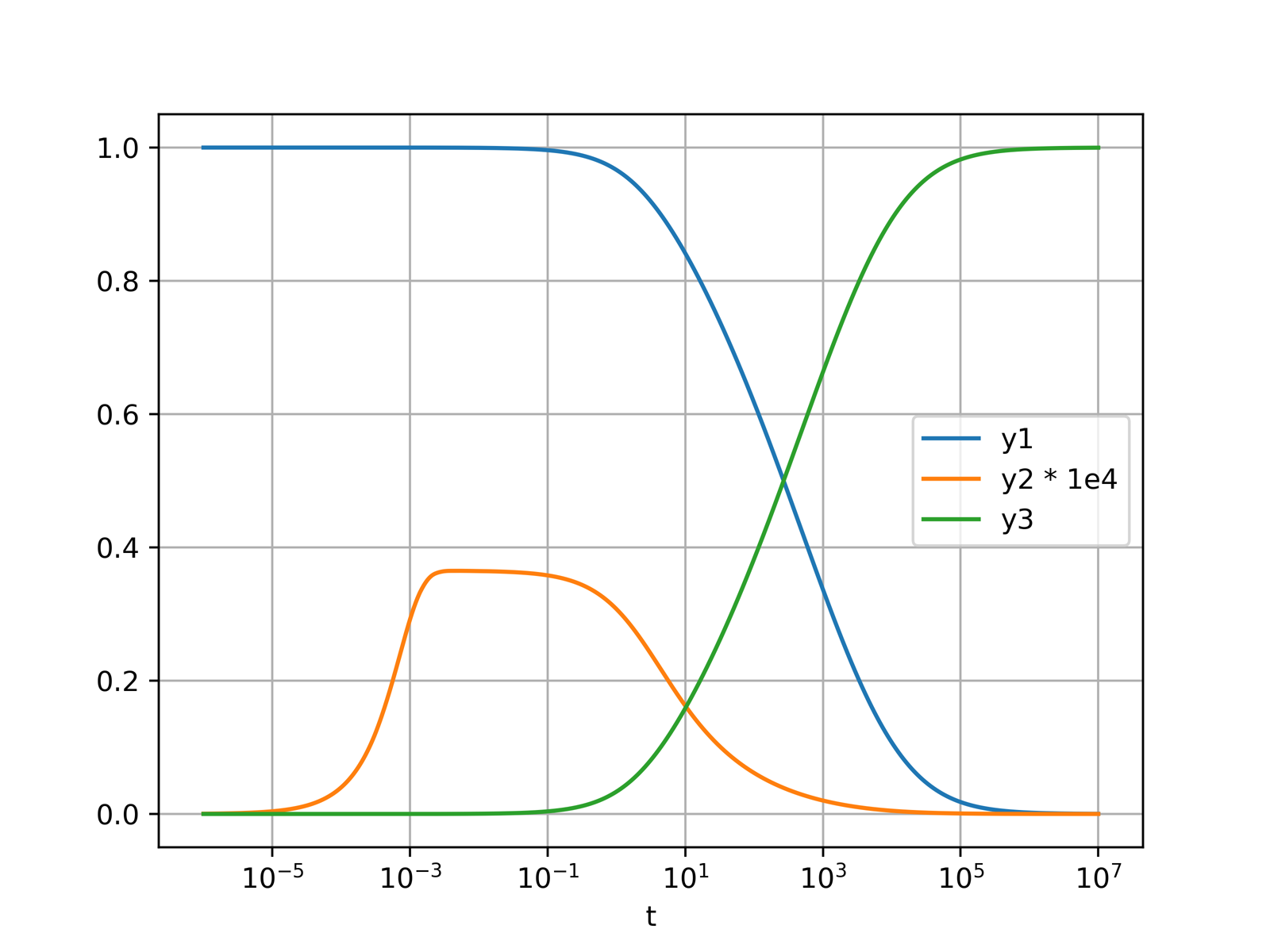
More examples are given in the examples directory, which includes

ordinary differential equations (ODE's)
differential algebraic equations (DAE's)
implicit differential equations (IDE's)

Work-precision

In order to investigate the work precision of the implemented solvers, we use different DAE examples with differentiation index 1, 2 and 3 as well as IDE example.

Index 1 DAE - Brenan

Brenan's index 1 problem is described by the system of differential algebraic equations

$$ \begin{aligned} \dot{y}_1 - t \dot{y}_2 &= y_1 - (1 + t) y_2 \\ 0 &= y_2 - \sin(t) . \end{aligned} $$

For the consistent initial conditions $t_0 = 0$, $y_1(t_0) = 1$, $y_2(t_0) = 0$, $\dot{y}_1 = -1$ and $\dot{y}_2 = 1$, the analytical solution is given by $y_1(t) = e^{-t} + t \sin(t)$ and $y_2(t) = \sin(t)$.

This problem is solved for $atol = rtol = 10^{-(1 + m / 4)}$, where $m = 0, \dots, 45$. The resulting error at $t_1 = 10$ is compared with the elapsed time of the used solvers in the figure below. For reference, the work-precision diagram of sundials IDA solver is also added. Note that the elapsed time is scaled by a factor of 100 since the sundials C-code is way faster.

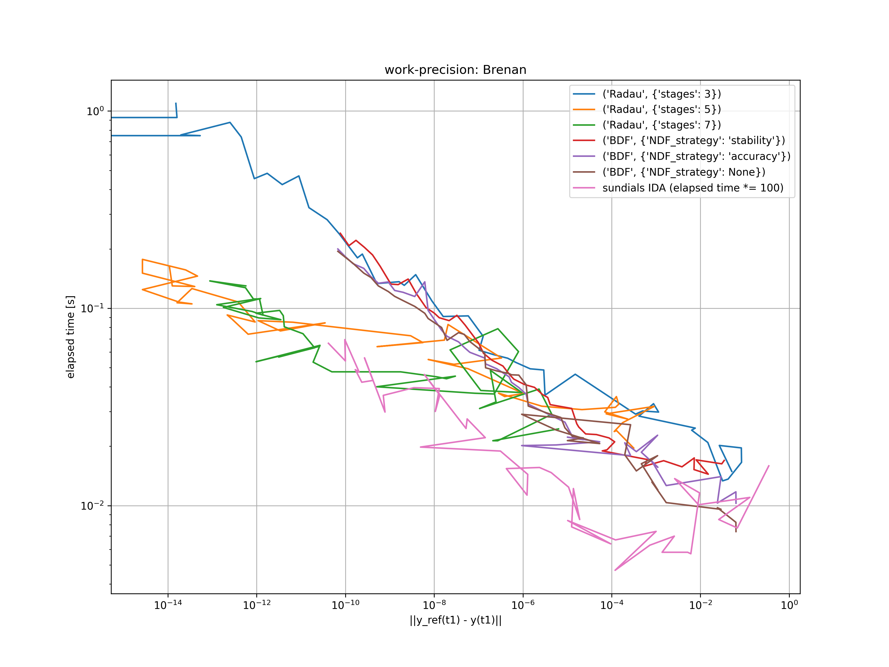
Clearly, the family of Radau IIA methods outplay the BDF/NDF methods for low tolerances. For medium to high tolerances, both methods are appropriate.

Index 2 DAE - knife edge

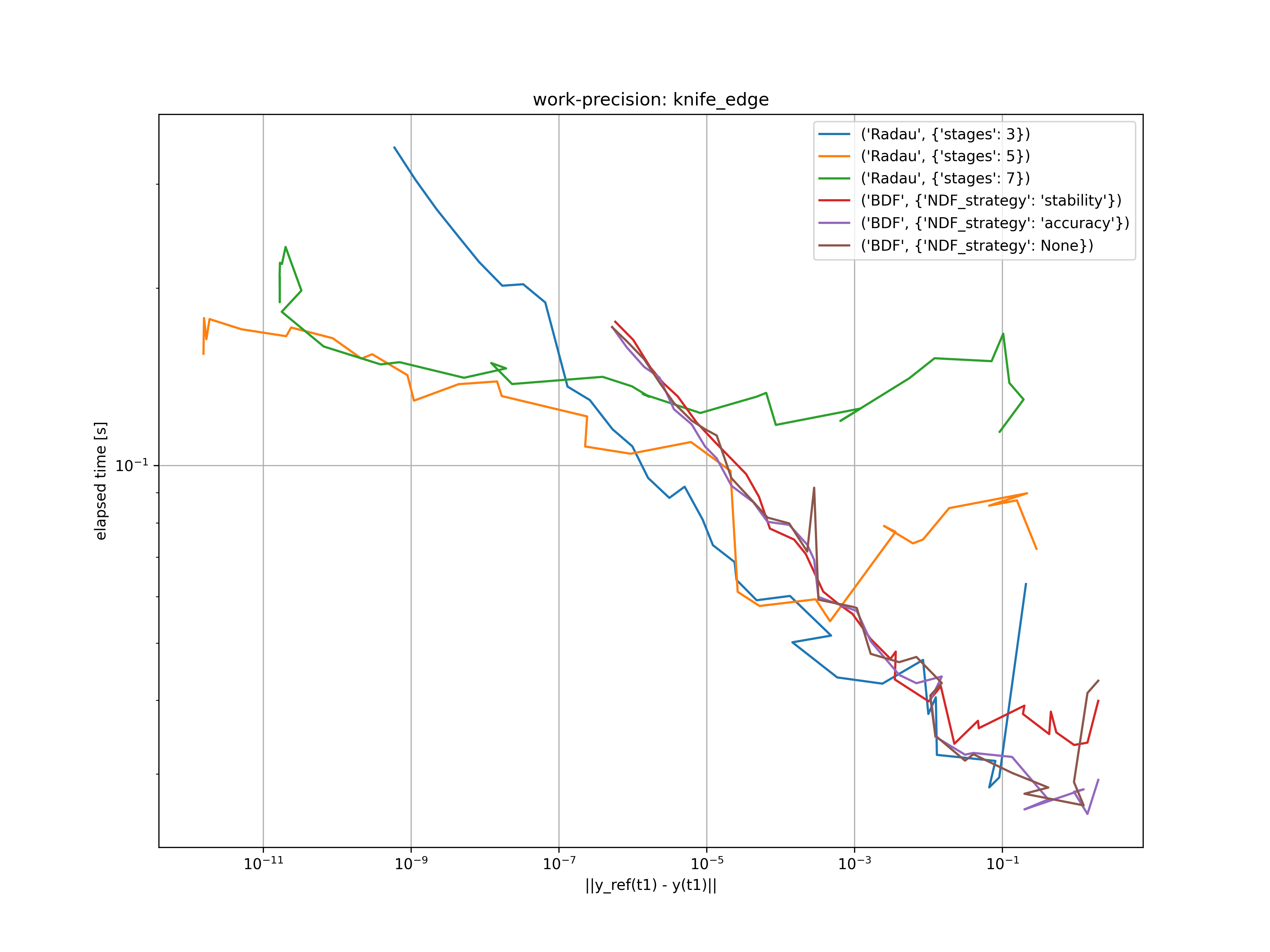
The knife edge index 2 problem is a simple mechanical example with nonholonomic constraint. It is described by the system of differential algebraic equations

$$ \begin{aligned} \dot{x} &= u \\ \dot{y} &= v \\ \dot{\varphi} &= \omega \\ m \dot{u} &= m g \sin\alpha + \sin\varphi \lambda \\ m \dot{v} &= -\cos\varphi \lambda \\ J \dot{\omega} &= 0 \\ 0 &= u \sin\varphi - v \cos\varphi . \end{aligned} $$

Since the implemented solvers are designed for index 1 DAE's we have to perform some sort of index reduction. Therefore, we transform the semi-explicit form into a general form as proposed by Gear. The resulting index 1 system is given as

$$ \begin{aligned} \dot{x} &= u \\ \dot{y} &= v \\ \dot{\varphi} &= \omega \\ m \dot{u} &= m g \sin\alpha + \sin\varphi \dot{\Lambda} \\ m \dot{v} &= -\cos\varphi \dot{\Lambda} \\ J \dot{\omega} &= 0 \\ 0 &= u \sin\varphi - v \cos\varphi . \end{aligned} $$

For the initial conditions $t_0 = 0$, $x(t_0) = \dot{x}(t_0) = y(t_0) = \dot{y}(t_0) = \varphi(t_0) = 0$ and $\dot{\varphi}(t_0) = \Omega$, a closed form solution is given by

$$ \begin{aligned} x(t) &= \frac{g \sin\alpha}{2 \Omega^2} \sin^2(\Omega t) \\ y(t) &= \frac{g \sin\alpha}{2 \Omega^2} \left(\Omega t - \frac{1}{2}\sin(2 \Omega t)\right) \\ \varphi(t) &= \Omega t \\ u(t) &= \frac{g \sin\alpha}{\Omega} \sin(\Omega t) \cos(\Omega t) \\ v(t) &= \frac{g \sin\alpha}{2 \Omega} \left(1 - \cos(2 \Omega t)\right) = \frac{g \sin\alpha}{\Omega} \sin^2(\Omega t) \\ \omega(t) &= \Omega \\ \Lambda(t) &= \frac{2g \sin\alpha}{\Omega} (\cos(\Omega t) - 1) , % (2 * m * g * salpha / Omega) * (np.cos(Omega * t) - 1) \end{aligned} $$

with the Lagrange multiplier $\dot{\Lambda}(t) = - 2g \sin\alpha \sin(\Omega t)$.

This problem is solved for $atol = rtol = 10^{-(1 + m / 4)}$, where $m = 0, \dots, 32$. The resulting error at $t_1 = 2 \pi / \Omega$ is compared with the elapsed time of the used solvers in the figure below.

Index 3 DAE - Arevalo

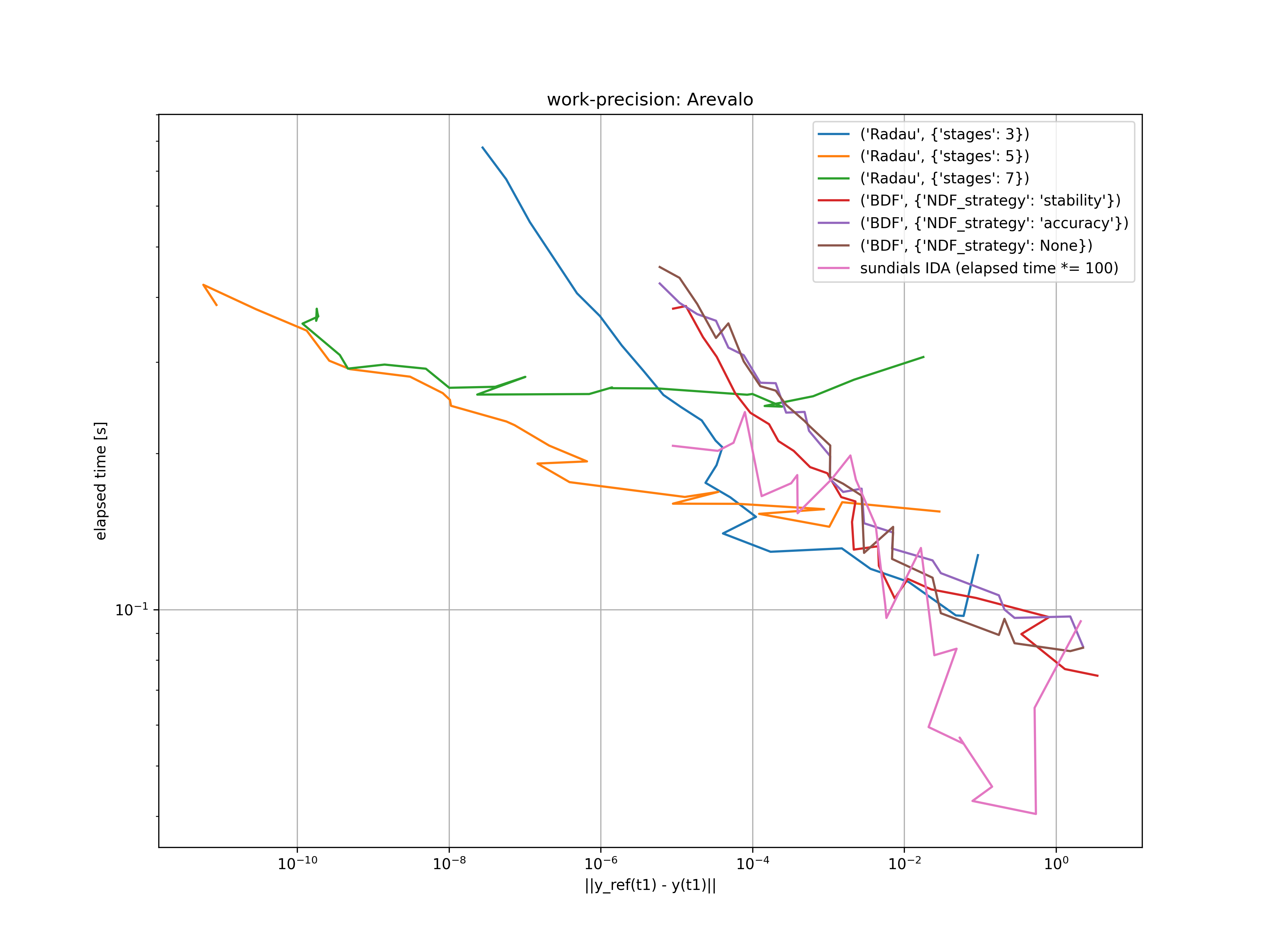
Arevalo's index 3 problem describes the motion of a particle on a circular track. It is described by the system of differential algebraic equations

$$ \begin{aligned} \dot{x} &= u \\ \dot{y} &= v \\ \dot{u} &= 2 y + x \lambda \\ \dot{v} &= -2 x + y \lambda \\ 0 &= x^2 + y^2 - 1 . \end{aligned} $$

Since the implemented solvers are designed for index 1 DAE's we have to perform some sort of index reduction. Therefore, we use the stabilized index 1 formulation of Hiller and Anantharaman. The resulting index 1 system is given as

$$ \begin{aligned} \dot{x} &= u + x \dot{\Gamma} \\ \dot{y} &= v + y \dot{\Gamma} \\ \dot{u} &= 2 y + x \dot{\Lambda} \\ \dot{v} &= -2 x + y \dot{\Lambda} \\ 0 &= x u + y v \\ 0 &= x^2 + y^2 - 1 . \end{aligned} $$

The analytical solution to this problem is given by

$$ \begin{aligned} x(t) &= \sin(t^2) \\ y(t) &= \cos(t^2) \\ u(t) &= 2 t \cos(t^2) \\ v(t) &= -2 t \sin(t^2) \\ \Lambda(t) &= -\frac{4}{3} t^3 \\ \Gamma(t) &= 0 , \end{aligned} $$

with the Lagrange multipliers $\dot{\Lambda} = -4t^2$ and $\dot{\Gamma} = 0$.

This problem is solved for $atol = rtol = 10^{-(3 + m / 4)}$, where $m = 0, \dots, 24$. The resulting error at $t_1 = 5$ is compared with the elapsed time of the used solvers in the figure below.

IDE - Weissinger

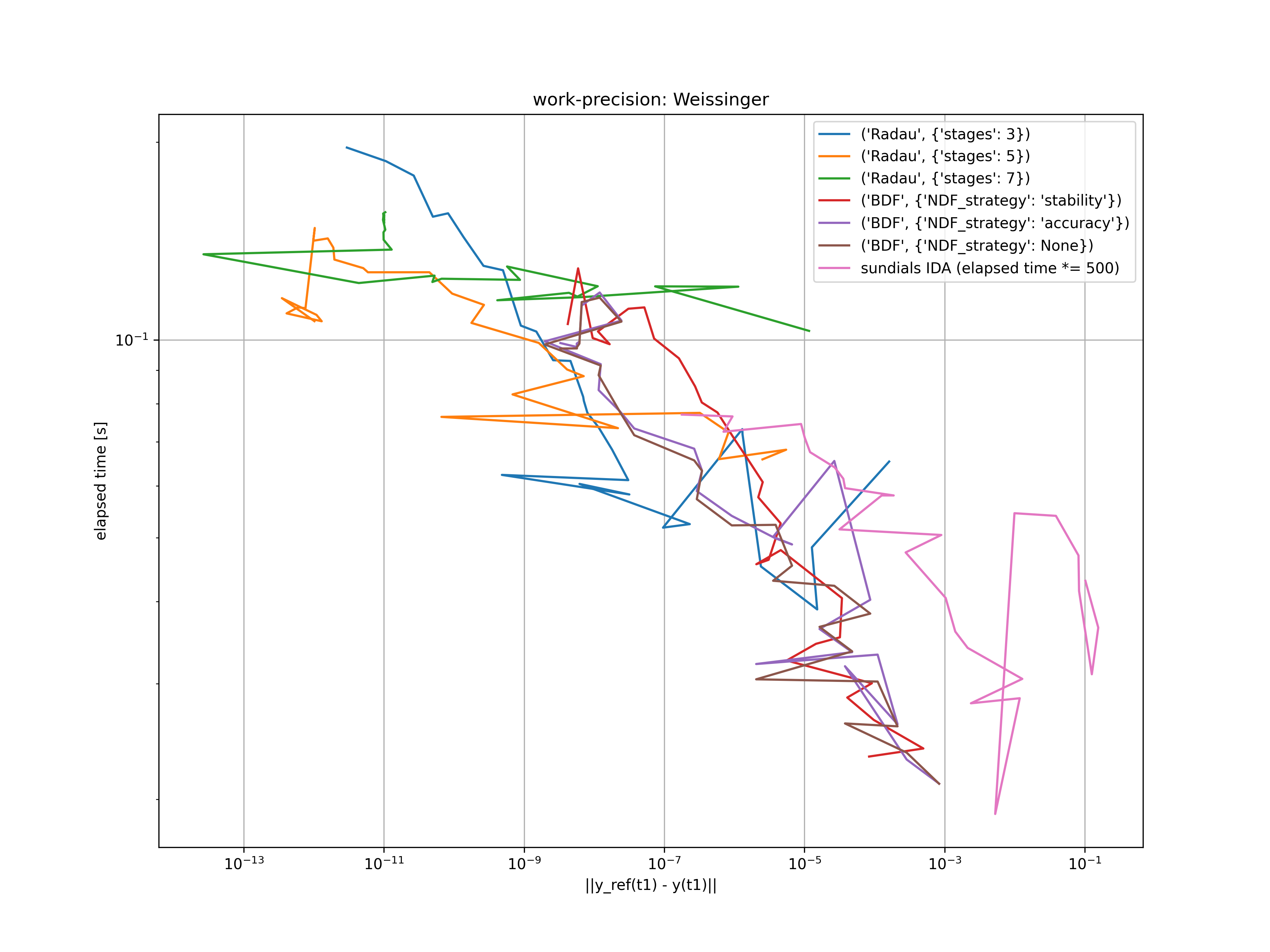
A simple example of an implicit differential equations is called Weissinger's equation

$$ t y^2 (\dot{y})^3 - y^3 (\dot{y}^2) + t (t^2 + 1) \dot{y} - t^2 y = 0 . $$

It has the analytical solution $y(t) = \sqrt{t^2 + \frac{1}{2}}$ and $\dot{y}(t) = \frac{t}{\sqrt{t^2 + \frac{1}{2}}}$.

Starting at $t_0 = \sqrt{1 / 2}$, this problem is solved for $atol = rtol = 10^{-(4 + m / 4)}$, where $m = 0, \dots, 28$. The resulting error at $t_1 = 10$ is compared with the elapsed time of the used solvers in the figure below.

Nonlinear index 1 DAE - Kvaernø

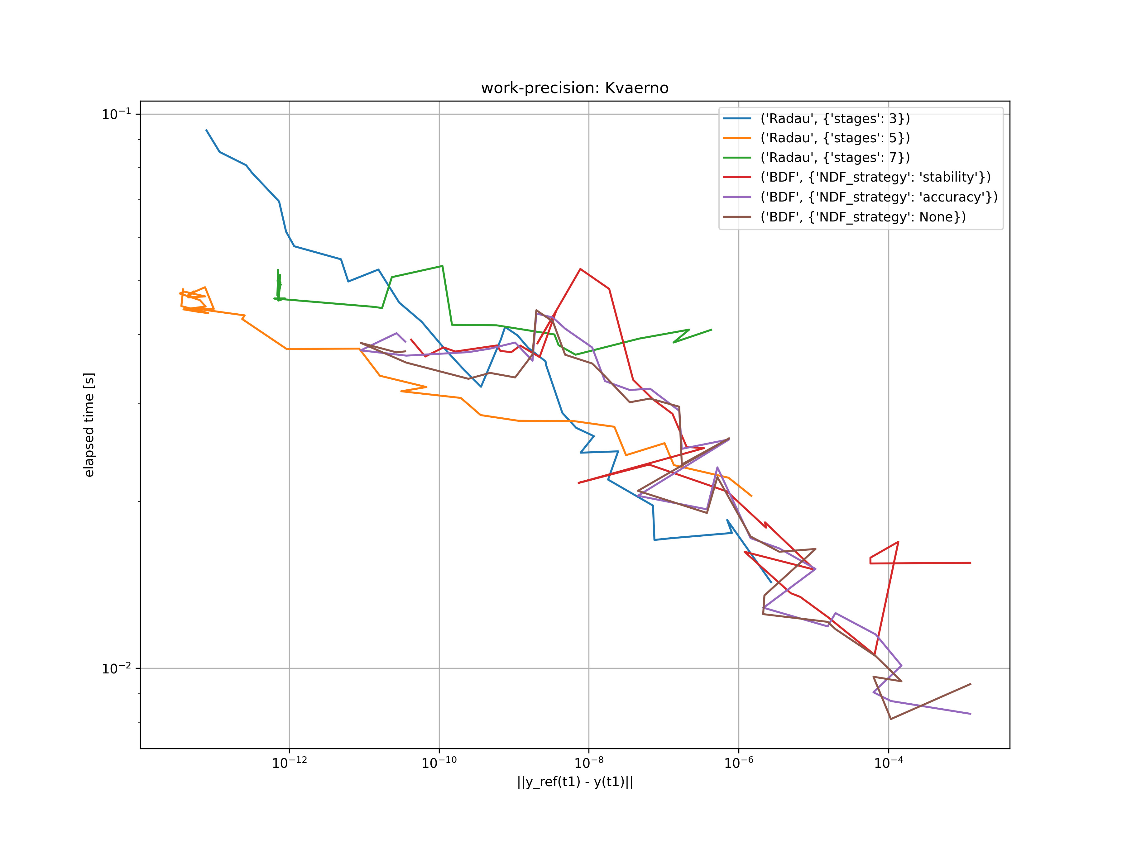
In a final example, an nonlinear index 1 DAE is investigated as proposed by Kvaernø. The system is given by

$$ \begin{aligned} (\sin^2(\dot{y}_1) + \sin^2(y_2)) (\dot{y}_2)^2 - (t - 6)^2 (t - 2)^2 y_1 e^{-t} &= 0 \\ (4 - t) (y_2 + y_1)^3 - 64 t^2 e^{-t} y_1 y_2 &= 0 , \end{aligned} $$

It has the analytical solution $y_1(t) = t^4 e^{-t}$, $y_2(t) = t^3 e^{-t} (4 - t)$ and $\dot{y}_1(t) = (4 t^3 - t^4) e^{-t}$, $y_2(t) = (-t^3 + (4 - t) 3 t^2 - (4 - t) t^3) e^{-t}$.

Starting at $t_0 = 0.5$, this problem is solved for $atol = rtol = 10^{-(4 + m / 4)}$, where $m = 0, \dots, 32$. The resulting error at $t_1 = 1$ is compared with the elapsed time of the used solvers in the figure below.

Install

An editable developer mode can be installed via

python -m pip install -e .[dev]

The tests can be started using

python -m pytest --cov

JonasBreuling/scipy_dae