Decomposition SHAP

Code accompanying Explaining the Model and Feature Dependencies by Decomposition of the Shapley Value.

SHAP values have become increasingly popular in recent years. However, it is (was) unclear how to apply them to datasets with dependent features. In our paper we provide a summary of the different options that arise and their motivations. Essentially, two popular SHAP implementations exist with followers on both sides: one that explains the model (Interventional SHAP [1], the regular shap implementation) and one that explain the model combined with the feature dependencies (Conditional SHAP [2]). We will illustrate that both options are valuable for different inferences with a simple example. Consider two binary dependent features $X_1$ and $X_2$, and a model which output is equal to the first feature, $f([X_1,X_2]) = X_1$. Now consider two different fictive settings:

	$X_1$	$X_2$	$f(\cdot)$	Interventional SHAP	Conditional SHAP	Decomposition SHAP
court	recidivist	race	future recidivism	✔️		✔️
hospital	high heart rate	obesity	heart attack		✔️	✔️

Given a certain sample, with SHAP we explain its output by determining what effect every feature value has towards the output. In the first setting $f$ is an indicator for the future recidivism of a convict. A convict $\boldsymbol{x}$ can demand an explanation of the algorithm involved in the courts decision. In this case the explanation should attribute $f([\boldsymbol{x}_1,\boldsymbol{x}_2])$ entirely to $\boldsymbol{x}_1$, showing absence of racial bias in the model. The second setting requires a different explanation. For patient $\boldsymbol{x}$ with a high heart attack risk, a good explanation should attribute part of $f([\boldsymbol{x}_1,\boldsymbol{x}_2])$ to $\boldsymbol{x}_2$, since changing $\boldsymbol{x}_2$ by losing weight could decrease the heart rate, which in term reduces the odds of having a heart attack according to the model. Note that this last attribution is solely due to the feature dependency.

Preferably, a good method should provide both inferences. Therefore, we propose to split up a SHAP value for a feature into a model corresponding (interventional) attribution and an attribution via other dependent features, allowing the end-user (e.g. convict or patient) to easily grasp the explanation of both the model and feature dependencies.

These attributions can be visualized through our modified force plots. For the simple toy example above, we explain $f(X_1=1,X_2=1) =1$.

We see that the convict's race has no interventional effect. Whether the patient is obese does have an output effect via its dependent feature high heart rate which is clearly shown in the explanation.

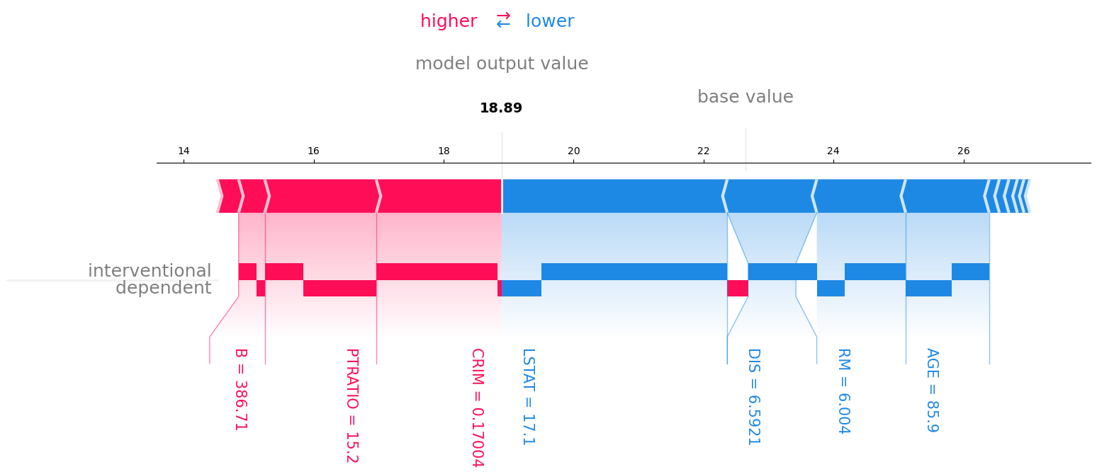
Furthermore, we can apply our method to the standard Boston Housing dataset and explain the prediction of a random forest model.

We see that the crime rate per capita ($\mathit{CRIM}$) being 0.17004 has a big positive effect on the median house price in this town, and the effect is largely interventional. This means that the $\mathit{CRIM}$ of this town has a strong effect on the output via its specific weights in the model. The pupil-teacher ratio $\mathit{PTRATIO}$ also has positive effect. A significant part of this effect is through its dependent features: it influences the distributions of the dependent features which in term increase the expected model output via their specific weights. We can also see that the model has a small racial bias: the interventional part of $B$ is non-zero.

Install instructions

clone the Github respository
install Conda environment (requires Conda): conda env create -f environment.yml

Usage

Let's illustrate the use of our toolbox with an example. We will use the Breast Cancer Wisconsin dataset and a XGBoost model to predict the cancer type. We will then explain the prediction of a test sample using Decomposition SHAP. The full code is available in example.py.

First load the data and train the model:

import numpy as np
import xgboost as xgb
from sklearn.datasets import load_breast_cancer
from sklearn.model_selection import train_test_split

from decomposition_shap.distributions import MultiGaussian
from decomposition_shap.force_dependent import force_dependent_plot
from decomposition_shap.kernel_dependent import DependentKernelExplainer

np.random.seed(0)

# Load Breast Cancer Wisconsin dataset
x, y = load_breast_cancer(return_X_y=True)
x_train, x_test, y_train, y_test = train_test_split(x, y, test_size=0.2)
    
# Fit a model
model = xgb.XGBClassifier(n_estimators=10)
model.fit(x_train, y_train)

Since we are computing data dependencies, an assumed data distribution is required. In this case we will use a multivariate Gaussian distribution. We can now explain the prediction of a test sample:

# Fit feature distribution (assumed Multivariate Gaussian)
dist = MultiGaussian(x_train)
# Note: custom distributions can also be defined see decomposition_shap/distribution.py

# Initialize explainer
explainer = DependentKernelExplainer(lambda d: model.predict(d, output_margin=True), x_train, dist.sample)
# Note: as with regular SHAP, usually it makes more sense to explain the logodds 'model.predict(d, output_margin=True)'
# instead of the class probabilities 'model.predict(d)'

# Explain the third test sample
sample_index = 3
shaps = explainer.shap_values(x_test[sample_index])  # returns array of conditional SHAP values + interventional effects

The SHAP values can be visualized using the force_dependent_plot function:

data = load_breast_cancer()
# With link='logit' the logodds are shown under the axis, and the probability is shown above the axis
fig = force_dependent_plot(np.mean(model.predict(x_train)), shaps, features=x_test[sample_index],
                       feature_names=data['feature_names'], link='logit', text_rotation=-90)  # returns plt.gcf()
fig.savefig("example.png", bbox_inches="tight")

Files and important functions

\decomposition_shap\kernel_dependent.py holds functions that can compute interventional and dependent effects
- class DependentKernelExplainer explains output of any function for any situation by decomposing the Shapley value into an interventional and dependent effect. See code documentation for information on constructor arguments.
- function shap_values(...) estimates the SHAP values and interventional effects for a set of samples. See code documentation for information on arguments.
\decomposition_shap\force_dependent.py holds implementation of force plot visualizations with interventional and dependent effects
- function force_dependent_plot(...) visualizes the given SHAP values and interventional effects in a matplotlib force plot. See code documentation for information on arguments.
\decompostion_shap\distributions.py holds different implementations of assumed data distributions
\experiments has all code to do all experiments of the paper and generate all results
example.py has a simple example to illustrate the use of Decomposition SHAP
tests tests of the implemented code

Citation

If you use Decomposition SHAP in your research we would appreciate citing Explaining the Model and Feature Dependencies by Decomposition of the Shapley Value

References

[1] Janzing, D., Minorics, L., & Blöbaum, P. (2020, June). Feature relevance quantification in explainable AI: A causal problem. In International Conference on artificial intelligence and statistics (pp. 2907-2916). PMLR.