This module provides common functions associated with antenna arrays. Currently it provides the creation of antenna array manifolds of ideal antennas and / or of measured steering vectors based on Look-up-Tables (LUT).
- Easy access to antenna array manifolds either ideal or real
- Create patterns
Install:
julia> ]
pkg> add PhasedArrayYou can either create an ideal manifold based on antenna positions and center frequency
using PhasedArray, StaticArrays
antenna_positions = 0.1904 / 4 *
    @SMatrix [1 -1  1 -1;
              1  1 -1 -1;
              0  0  0  0]
manifold = IdealManifold(1575420e3, antenna_positions)
doa = @SVector [0, 0, 1]
steer_vec = get_steer_vec(manifold, doa)or you can create a real manifold based on a measured LUT:
using PhasedArray, StaticArrays
manifold = RealManifold(lut, PhasedArray.NumAnts(4))
steer_vec = get_steer_vec(manifold, SVector(0, 0, 1))
The LUT can either be a 3D Array, where the first dimension holds the antenna channels, the second dimension the elevations and the third dimension the azimuths, or it can be a SVector of a matrices, where each matrix holds the elevations on the first dimension and the azimuths on the second dimension per antenna channel.
If you pass a 3D Array, you must also provide the NumAnts(num_ants) argument.
The interpolation can be set with the interpolation argument. The default one is Constant. You can change that to Linear or Quadratic, if you'd like to.
By default the LUT is normalized to its highest gain. If you don't want that, you can pass the argument normalize = false to the RealManifold function.
The function get_steer_vec has an optional third argument for a rotation matrix, if you'd like to rotate the Direction of Arrival (DoA) before looking up the steering vector.
This module also provides some helping functions, if you'd like to plot a pattern
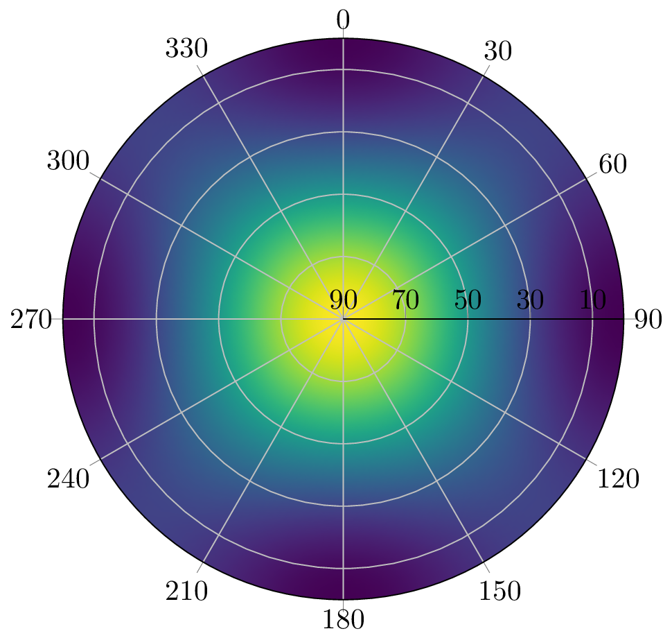
A 2D pattern can be generated with:
reduce_ant_function = norm
pattern = Pattern(manifold, reduce_ant_function, num_az = 360, num_el = 91, max_el = π / 2)
The reduce_ant_function can be any function, that reduces the antenna channels to a scalar real value.
This pattern can be plotted with Plots.jl in the following way:
using Plots
plot(pattern)
Alternatively you can plot it with PGFPlotsX:
using PGFPlotsX
@pgf PolarAxis(
    {
        ymin = 0,
        ymax = pattern.max_el * 180 / π,
        "colormap/viridis",
        "axis on top",
        "colorbar style={title=Amplification (dB)}",
        xticklabel = "{\$\\pgfmathparse{Mod(90-\\tick,360)}\\pgfmathprintnumber{\\pgfmathresult}\$}",
        yticklabel = "{\$\\pgfmathparse{90-\\tick}\\pgfmathprintnumber{\\pgfmathresult}\$}",
    },
    Plot3({surf, shader="interp"},
        Coordinates(pattern.azs .* 180 ./ π, pattern.els .* 180 ./ π, pattern.values')
    )
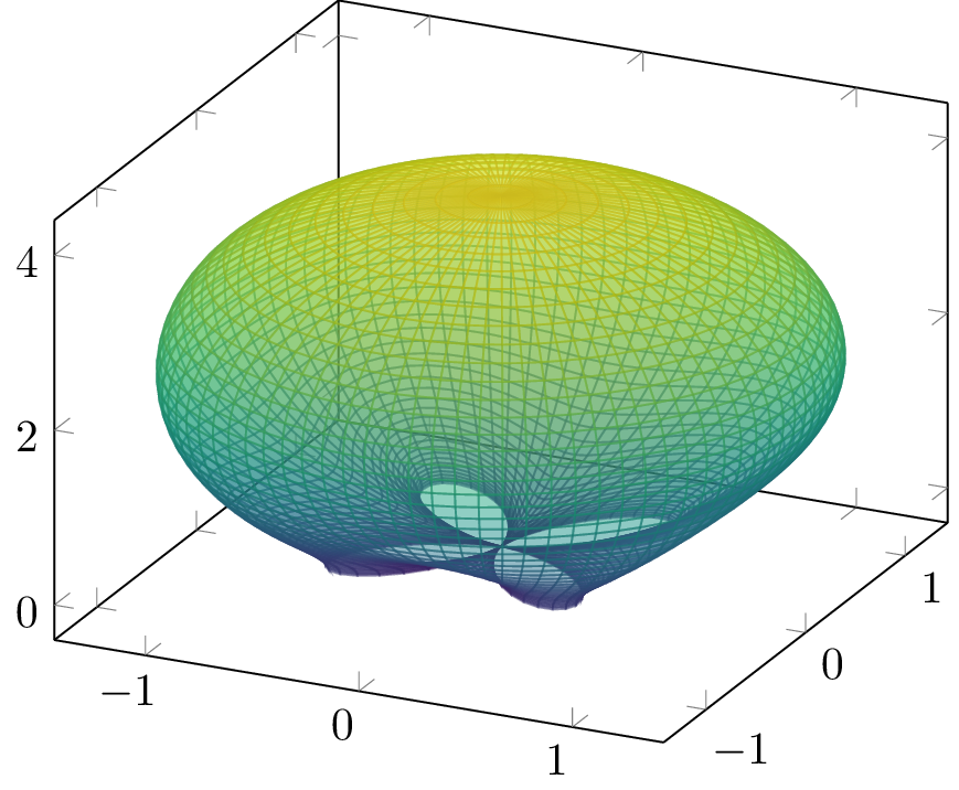
)If you'd like to plot a 3D figure, this can be done with the following code:
reduce_ant_function = norm
pattern = Pattern3D(manifold, reduce_ant_function, num_az = 360, num_el = 181, max_el = π)
Again, this can be plotted with Plots.jl:
using Plots
plot(pattern)
# If you use plotlyjs() you can also plot the gain correctly:
# plot(pattern, fill_z = pattern.gains)
Alternatively you can plots the pattern with PGFPlotsX in the following way:
using PGFPlotsX
@pgf Axis({"colormap/viridis"},
    Plot3({surf, "z buffer=sort", "opacity=0.5", "point meta=sqrt(x^2+y^2+z^2)"},
        Table([:x=>vec(pattern.X), :y=>vec(pattern.Y), :z=>vec(pattern.Z)]; scanlines = size(pattern.X,1))
    )
)MIT License

