fasster

An implementation of the FASSTER (Forecasting with Additive Switching of Seasonality, Trend and Exogenous Regressors) model in R. This model is designed to capture patterns of multiple seasonality in a state space framework by using state switching. The fasster package prioritizes flexibility, computational speed and accuracy to provide convenient tools for modelling, predicting and understanding high frequency time-series.

Installation

The development version can be installed from GitHub using:

# install.packages("devtools")
devtools::install_github("mitchelloharawild/fasster")

Usage

Model specification

fasster allows flexible model specification by allowing the user to specify the model structure with standard formula conventions.

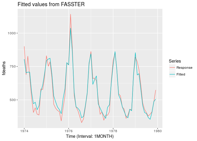
fasster(fdeaths ~ mdeaths) %>% ggfitted

Commonly used state space components can be added using the following convenience functions:

poly(n) to include an n-th order polynomial
seas(s) to include a seasonal factor of frequency s
trig(s, q) to include seasonal fourier terms of frequency s with q harmonics
arma(ar, ma) to include an ARMA term (where ar and ma are vectors of coefficients)
Exogenous regressors can be added by referring to their name

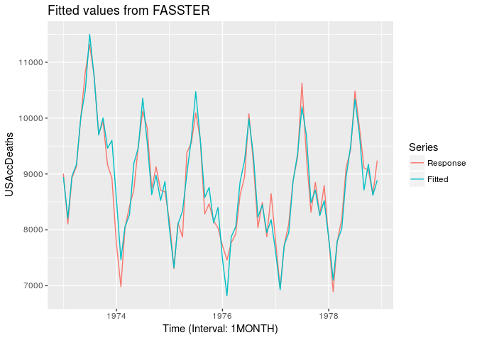
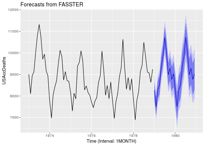
For example, to create a model with trend and monthly seasonality, you can use:

fit <- fasster(USAccDeaths ~ poly(1) + trig(12))
fit %>% ggfitted

The interface for creating a FASSTER model introduces a new formula construct, %S%, known as the switch operator. This allows modelling of more complex patterns such as multiple seasonality by modelling the components for each group seperately and switching between them.

fit_switch <- as_tsibble(taylor) %>%
  mutate(index = seq(ymd_h("2000-6-5 00"), by="30 mins", length.out=length(taylor)),
         DayType = ifelse(wday(index) %in% 2:6, "Weekday", "Weekend")) %>% 
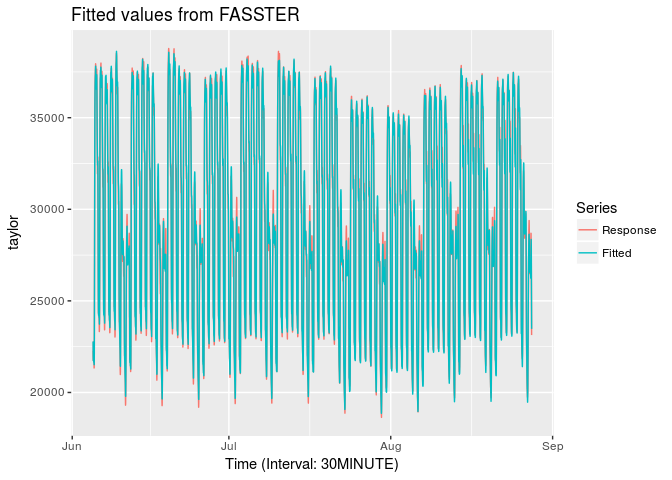
  fasster(taylor ~ DayType %S% (poly(1) + trig(48, 10))) 
fit_switch %>%
  ggfitted

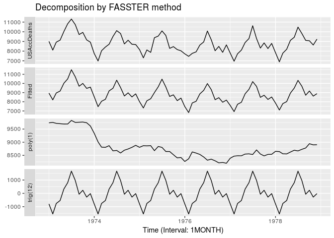
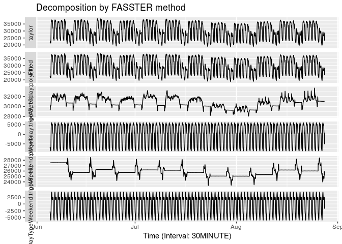
Decomposing

Fitted FASSTER models can be decomposed to provide a description of how the underlying states function. Decomposing a FASSTER model provides aggregates of its components such as trends and seasonalities.

These components can be plotted using the autoplot function on a fitted model:

fit %>% autoplot

fit_switch %>% autoplot

The tools made available by fasster are designed to integrate seamlessly with the tidyverse of packages, enabling familiar data manipulation and visualisation capabilities.

Forecasting

fasster conforms to the object structure from the forecast package, allowing common visualisation and analysis tools to be applied on FASSTER models.

library(forecast)
fit %>% accuracy
#>                     ME     RMSE      MAE        MPE     MAPE      MASE
#> Training set -23.10502 257.6256 190.2418 -0.3173936 2.204005 0.2956716
#>                   ACF1
#> Training set 0.1697722

fit %>% 
  forecast(h=24) %>%
  autoplot

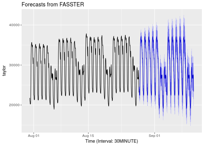
Like other forecasting functions, if additional information is required (such as future state switching), it can be provided via the newdata argument.