This is a collection of option pricing functions for a course in financial derivatives. The names of the functions mostly match those in my book Derivatives Markets, which explains the package name. This should be useful for students comfortable with R. In any case, I hope it will be helpful for instructors.
There are of course other option pricing packages in R, notably RQuantLib and fOptions. I don’t add significant pricing functionality to those. This package does, however, have a few aspects that might be unique, which I describe below: calculation of greeks; display of binomial formula output and trees; and a quincunx function.
The package includes functions for computing
-
Black-Scholes prices and greeks for European options
-
Option pricing and plotting using the binomial model
-
Barrier options
-
Compound options
-
Pricing of options with jumps using the Merton model
-
Analytical and Monte Carlo pricing of Asian options
-
Simulation of stock price paths, with and without jumps
Calculation of Greeks
The function greeks() accepts an option pricing function call as an
argument, and returns a vectorized set of greeks for any pricing
function that uses the input names standard in the package (i.e., the
asset price is s, the volatility is v, the interest rate is r, the
dividend yield is d, and the time to maturity is tt).
As an example, the following calculation will produce the full
complement of greeks for a call, for each of three strike prices. You
can access the delta values, for example, using x['Delta', ].
x1 <- greeks(bscall(s=40, k=c(35, 40, 45), v=0.3, r=0.08, tt=0.25, d=0))
x1
             bscall_35   bscall_40   bscall_45
Premium     6.13481997  2.78473666  0.97436823
Delta       0.86401619  0.58251565  0.28200793
Gamma       0.03636698  0.06506303  0.05629794
Vega        0.04364029  0.07807559  0.06755753
Rho         0.07106457  0.05128972  0.02576487
Theta      -0.01340407 -0.01733098 -0.01336419
Psi        -0.08640162 -0.05825156 -0.02820079
Elasticity  5.63352271  8.36726367 11.57705764
There is a new complete option which produces one row containing all
inputs and outputs for each case. The option long=TRUE produces the
same output in long form.
x2 <- greeks(bscall(s=40, k=c(35, 40, 45), v=0.3, r=0.08, tt=0.25, d=0),
             complete=TRUE)
x2
   s  k   v    r   tt d funcname   Premium     Delta       Vega        Rho
1 40 35 0.3 0.08 0.25 0   bscall 6.1348200 0.8640162 0.04364029 0.07106457
2 40 40 0.3 0.08 0.25 0   bscall 2.7847367 0.5825156 0.07807559 0.05128972
3 40 45 0.3 0.08 0.25 0   bscall 0.9743682 0.2820079 0.06755753 0.02576487
        Theta         Psi     Elast      Gamma
1 -0.01340407 -0.08640162  5.633523 0.03636698
2 -0.01733098 -0.05825156  8.367264 0.06506303
3 -0.01336419 -0.02820079 11.577058 0.05629794

x3 <- greeks(bscall(s=40, k=c(35, 40, 45), v=0.3, r=0.08, tt=0.25, d=0),
             long=TRUE)
x3
    s  k   v    r   tt d funcname   greek       value
1  40 35 0.3 0.08 0.25 0   bscall Premium  6.13481997
2  40 40 0.3 0.08 0.25 0   bscall Premium  2.78473666
3  40 45 0.3 0.08 0.25 0   bscall Premium  0.97436823
4  40 35 0.3 0.08 0.25 0   bscall   Delta  0.86401619
5  40 40 0.3 0.08 0.25 0   bscall   Delta  0.58251565
6  40 45 0.3 0.08 0.25 0   bscall   Delta  0.28200793
7  40 35 0.3 0.08 0.25 0   bscall    Vega  0.04364029
8  40 40 0.3 0.08 0.25 0   bscall    Vega  0.07807559
9  40 45 0.3 0.08 0.25 0   bscall    Vega  0.06755753
10 40 35 0.3 0.08 0.25 0   bscall     Rho  0.07106457
11 40 40 0.3 0.08 0.25 0   bscall     Rho  0.05128972
12 40 45 0.3 0.08 0.25 0   bscall     Rho  0.02576487
13 40 35 0.3 0.08 0.25 0   bscall   Theta -0.01340407
14 40 40 0.3 0.08 0.25 0   bscall   Theta -0.01733098
15 40 45 0.3 0.08 0.25 0   bscall   Theta -0.01336419
16 40 35 0.3 0.08 0.25 0   bscall     Psi -0.08640162
17 40 40 0.3 0.08 0.25 0   bscall     Psi -0.05825156
18 40 45 0.3 0.08 0.25 0   bscall     Psi -0.02820079
19 40 35 0.3 0.08 0.25 0   bscall   Elast  5.63352271
20 40 40 0.3 0.08 0.25 0   bscall   Elast  8.36726367
21 40 45 0.3 0.08 0.25 0   bscall   Elast 11.57705764
22 40 35 0.3 0.08 0.25 0   bscall   Gamma  0.03636698
23 40 40 0.3 0.08 0.25 0   bscall   Gamma  0.06506303
24 40 45 0.3 0.08 0.25 0   bscall   Gamma  0.05629794
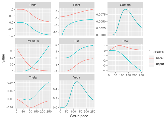
The following computes and plots all call and put Greeks for 500 options:
library(derivmkts)
library(ggplot2)
Registered S3 methods overwritten by 'ggplot2':
  method         from
  [.quosures     rlang
  c.quosures     rlang
  print.quosures rlang
s <- 100; r <- 0.08; v <- 0.30; tt <- 2; d <- 0
k <- seq(.5, 250, by=.5)
yc <- greeks(bscall(s, k, v, r, tt, d), long=TRUE)
yp <- greeks(bsput(s, k, v, r, tt, d), long=TRUE)
ggplot(rbind(yc, yp), aes(x=k, y=value, color=funcname)) +
    geom_line() +
    labs(x='Strike price') +
    facet_wrap(~ greek, scales='free_y')
Simulating stock prices
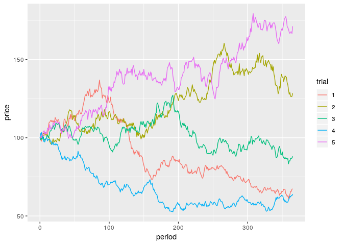
The simprice function produces simulated price paths, with output
either in wide or long form.
s <- simprice(s0 = 100, v = 0.3, r = 0.08, tt = 1, d = 0, trials = 5,
              periods = 365, jump = FALSE, long = TRUE, seed = 1)
ggplot(s, aes(x = period, y = price, color = trial)) +
    geom_line()
Binomial calculations
binomopt
By default the binomopt function returns the price of an American call. In adddition:
-
putopt=TRUEreturns the price of an American put. -
returngreeks=TRUEreturns a subset of the Greeks along with the binomial parameters. -
returntrees=TRUEreturns as a list all of the above plus the full binomial tree ($stree), the probability of reaching each node ($probtree), whether or not the option is exercised at each node ($exertree), and the replicating portfolio at each node ($deltatree and $bondtree).
Here is an example illustrating everything that the binomopt function
can return:
x <- binomopt(41, 40, .3, .08, 1, 0, 3, putopt=TRUE, american=TRUE,
              returntrees=TRUE)
x
$price
   price
3.292948

$greeks
       delta        gamma        theta
-0.331656818  0.037840906 -0.005106465

$params
         s          k          v          r         tt          d
41.0000000 40.0000000  0.3000000  0.0800000  1.0000000  0.0000000
     nstep          p         up         dn          h
 3.0000000  0.4568067  1.2212461  0.8636926  0.3333333

$oppricetree
         [,1]      [,2]     [,3]      [,4]
[1,] 3.292948 0.7409412 0.000000  0.000000
[2,] 0.000000 5.6029294 1.400911  0.000000
[3,] 0.000000 0.0000000 9.415442  2.648727
[4,] 0.000000 0.0000000 0.000000 13.584345

$stree
     [,1]     [,2]     [,3]     [,4]
[1,]   41 50.07109 61.14913 74.67813
[2,]    0 35.41139 43.24603 52.81404
[3,]    0  0.00000 30.58456 37.35127
[4,]    0  0.00000  0.00000 26.41565

$probtree
     [,1]      [,2]      [,3]       [,4]
[1,]    1 0.4568067 0.2086723 0.09532291
[2,]    0 0.5431933 0.4962687 0.34004825
[3,]    0 0.0000000 0.2950590 0.40435476
[4,]    0 0.0000000 0.0000000 0.16027409

$exertree
      [,1]  [,2]  [,3]  [,4]
[1,] FALSE FALSE FALSE FALSE
[2,] FALSE FALSE FALSE FALSE
[3,] FALSE FALSE  TRUE  TRUE
[4,] FALSE FALSE FALSE  TRUE

$deltatree
           [,1]        [,2]       [,3]
[1,] -0.3316568 -0.07824964  0.0000000
[2,]  0.0000000 -0.63298582 -0.1712971
[3,]  0.0000000  0.00000000 -1.0000000

$bondtree
         [,1]      [,2]      [,3]
[1,] 16.89088  4.658986  0.000000
[2,]  0.00000 28.017840  8.808828
[3,]  0.00000  0.000000 38.947430
binomplot
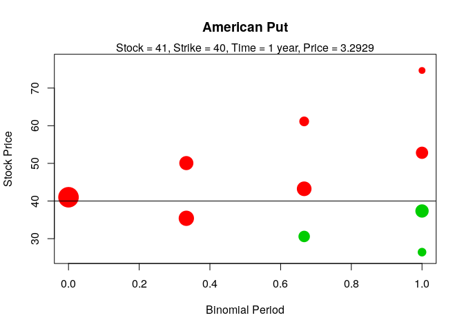
This function plots the binomial tree, providing a visual depiction of the nodes, the probability of reaching each node, and whether exercise occurs at that node.
binomplot(41, 40, .3, .08, 1, 0, 3, putopt=TRUE, american=TRUE)Galton board or quincunx
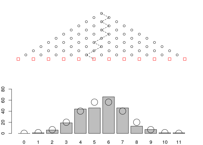
The Galton board is a pegboard that illustrates the central limit theorem. Balls drop from the top and randomly fall right or left, providing a physical simulation of a binomial distribution. (My physicist brother-in-law tells me that real-life Galton boards don’t typically generate a normal distribution because, among other things, balls acquire momentum in the direction of their original travel. The distribution is thus likely to be fatter-tailed than normal.)
You can see the Galton board in action with quincunx():
quincunx(n=11, numballs=250, delay=0, probright=0.5)Feedback
Please feel free to contact me with bug reports or suggestions. Best would be to file an issue on Github, but email is fine as well.


