Table of Contents:
This repository aims to demonstrate how to extract the fringe contrast from an interferogram and calculate the temporal decay of the first-order correlation function g(1)(t). The code was developed by Konstantinos Orfanakis and Dr Hamid Ohadi at the University of St Andrews and was extensively used for our first publication (Phys. Rev. B 103, 235313 (2021)).
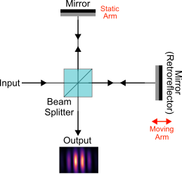
This experiment investigates the temporal coherence of an optically trapped exciton-polariton condensate. For this purpose, we utilise a Michelson interferometer in the mirror-retroreflector configuration (See Fig. 1). By varying the position of the moving arm (where a retroreflector is used for reflecting the beam) and superimposing the image from each arm, we form interferograms for various time delays.
Figure 1: Schematic of the interferometer setup.
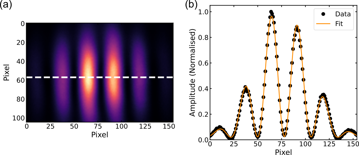
A line profile in the centre of the interferogram can be fit by a Gaussian function (the condensate mode profile) multiplied by a cosine to acquire the fringe contrast (see Fig. 2). The exact equation is the following:
Where parameters A, x0, and w are the amplitude, the centre, and the width of the Gaussian, respectively. The parameter α corresponds to the fringe contrast, k to the wavenumber, φ to the phase, and ct to a constant.
Figure 2: (a) Example of an interferogram. (b) Horizontal line profile across the white dashed line of the interference pattern in (a). The orange line shows the theoretical fit.
The fringe contrast is equal to the magnitude of the first-order correlation function |g(1)(t)|, where t is the time delay.
To acquire the temporal dependence of the correlation function, we record the fringe contrast while changing the time delay. We average over several (usually five) realisations for each time delay.
The experimental data are saved in the Hierarchical Data Format (HDF) as H5 files. Each interferogram is saved as a separate frame in this H5 file. A frame contains a 2D array corresponding to the interferogram image plus some extra information, called attributes (e.g. position of the moving arm, the exact time of the measurement, etc.).
In our case, we are only interested in the 2D image and the position of the moving arm. A pythonic interface to the HDF data format is provided by the h5py package.
Due to its size (105 MB), the file used in this tutorial cannot be uploaded on GitHub. It accessible through Dropbox. The dataset used for Phys. Rev. B 103, 235313 (2021) is available through the University of St Andrews.
Python Version: 3.10.2
Jupyter Notebook Version: 6.4.8
Packages: h5py (3.6.0), NumPy (1.22.2), Matplotlib (3.5.1), LMfit (1.0.3), SciPy (1.8.0), Pandas (1.4.1), tqdm (4.62.3)
If you have any feedback or ideas to improve this project, feel free to contact me via:


