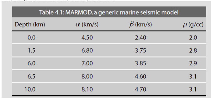
Consider MARMOD, a velocity-versus-depth model, which is typical of much of the oceanic crust (Table 4.1). Linear velocity gradients are assumed to exist at intermediate depths in the model; for example, the P velocity at 3.75 km is 6.9 km/s. Write a computer program to trace rays through this model:
and produce a P-wave T(X) curve, using 100 values of the ray parameter p equally spaced between 0.1236 and 0.2217 s/km. You will find it helpful to use subroutine LAYERXT (provided in Fortran in Appendix D and in the supplemental web material as a Matlab script), which gives dx and dt as a function of p for layers with linear velocity gradients. Your program will involve an outer loop over ray parameter and an inner loop over depth in the model. For each ray, set x and t to zero and then, starting with the surface layer and proceeding downward, sum the contributions, dx and dt, from LAYERXT for each layer until the ray turns. This will give x and t for the ray from the surface to the turning point. Multiply by two to obtain the total surface-to-surface values of X(p) and T(p). Now produce plots of: (a) T(X) plotted with a reduction velocity of 8 km/s, (b) X(p), and (c) τ(p). On each plot, label the prograde and retrograde branches.
