The data is a SQLite database, using DBI and dbplyr to query the database. The dataset is downloaded from Kaggle
library(DBI)
# Create an ephemeral in-memory RSQLite database
con <- dbConnect(RSQLite::SQLite(), "./database.sqlite")
reviews <- tbl(con, "reviews")
artists <- tbl(con, "artists")
content <- tbl(con, "content")
genres <- tbl(con, "genres")
years <- tbl(con, "years")allContent <- reviews %>%
inner_join(content, by=c("reviewid"="reviewid")) %>%
arrange(desc(pub_year)) %>%
select(reviewid, title, artist, score, author, author_type, content, pub_year, best_new_music) %>%
distinct() %>%
collect()
allContent1 <- allContent %>%
mutate(best_new_music=as.factor(best_new_music)) %>%
filter(pub_year>=2003)There are over 18000 reivews in the data. With limited computation power for text mining, we can only use a subset of the data. Here, I selected 2000 samples, 943 of them are best_new_music, rest are not. The best_new_music class is also balanced this way.
set.seed(1234)

bestNew <- allContent1 %>%
  filter(best_new_music=="1")

notBest <- allContent1 %>%
  filter(best_new_music == "0")

notBestIndex <- sample(1:nrow(notBest), 1000, replace= FALSE)
notBestSample <- notBest[notBestIndex,]

sample <- rbind(bestNew, notBestSample)Let's first see the high frequency words in reviews in a wordcloud.
reviewContent <- sample %>%
  mutate(content = tolower(content),
         content = lemmatize_strings(content),
         content = str_replace_all(content, "\\-", " "),
         content = stripWhitespace(content),
         content = removeNumbers(content))

mystopwords <- c("song", "album", "music", "track", "record", "sound","release", "much", "can")

tokens <-  reviewContent %>%
  unnest_tokens(word, content) %>%
  anti_join(stop_words) %>%
  filter(!(word %in% mystopwords)) %>%
  count(word) %>%
  mutate(freq = n/sum(n)) %>%
  top_n(n = 50, wt = freq)

tokens %>%
  ggplot(aes(label = word, size = freq, color = word))+
  geom_text_wordcloud_area()+
  scale_size_area(max_size = 20)+
  theme_minimal()
The frequent words in Pitchfork's reviews are mostly about genres, feelings and some musical terms. Very standard words you expect to see in music reviews.
reviewSenti = sentiment(get_sentences(allContent),
          polarity_dt = lexicon::hash_sentiment_jockers,
          valence_shifters_dt = lexicon::hash_valence_shifters)

reviewSenti1 = reviewSenti %>%
  group_by(reviewid) %>%
  summarize(sentiment = mean(sentiment))
Add sentiments back to our data frame. And remove some unimportant words
sample1 <- reviewContent %>%
  inner_join(reviewSenti1) %>%
  mutate(content = removeWords(content, mystopwords)) %>%
  filter(reviewid != 10497) # this review does not have content
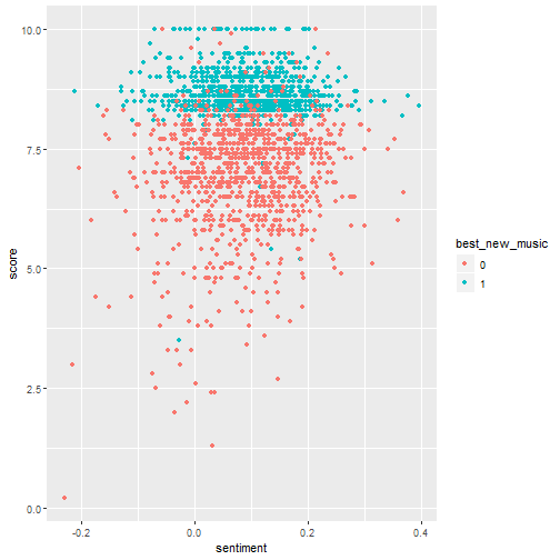
sample1 %>%
ggplot(aes(x=sentiment, y = score, color = best_new_music))+
geom_point()There is no visibal relationship between score and sentiment. But we can see the threshod in score for best new music.
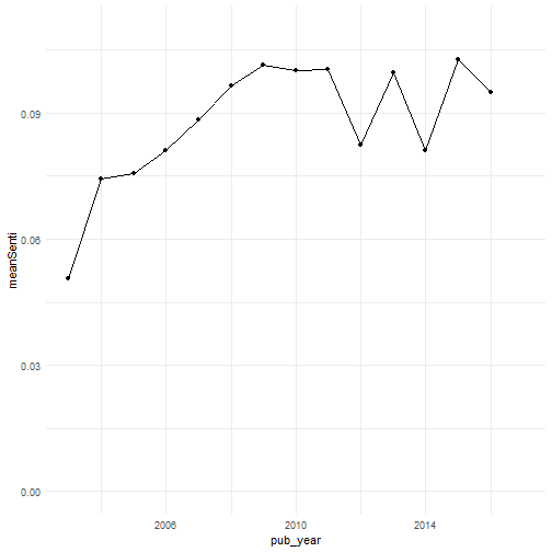
sample1 %>%
  group_by(pub_year) %>%
  summarize(meanSenti = mean(sentiment)) %>%
  ggplot(aes(x=pub_year, y = meanSenti))+
  geom_line()+
  geom_point()+
  ylim(0,0.11)+
  theme_minimal()
The review sentiment was climbing up before 2010. And went up and down after 2010. But it is varying in a small range.
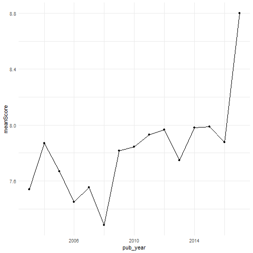
sample1 %>%
  group_by(pub_year) %>%
  summarize(meanScore = mean(score)) %>%
  ggplot(aes(x = pub_year, y = meanScore))+
  geom_line()+
  geom_point()+
  theme_minimal()
Again, 2010 seems to be a dividing point for scores.
library(stm)
predictorText = textProcessor(documents = sample1$content,
                          metadata = sample1,
                          stem = FALSE)
## Building corpus...
## Converting to Lower Case...
## Removing punctuation...
## Removing stopwords...
## Removing numbers...
## Creating Output...
pfPrep = prepDocuments(documents = predictorText$documents,
                               vocab = predictorText$vocab,
                               meta = predictorText$meta)
## Removing 18277 of 41296 terms (18277 of 658465 tokens) due to frequency
## Your corpus now has 1942 documents, 23019 terms and 640188 tokens.
kTest = searchK(documents = pfPrep$documents,
             vocab = pfPrep$vocab,
             K = c(3, 4, 5, 7, 10), verbose = FALSE)

#png(file = "./pfktest2.png", width = 800, height = 600)
plot(kTest)
#dev.off()
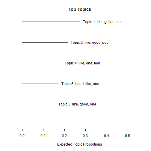
Choose 5 as the number of topics.
topics5 = stm(documents = pfPrep$documents,
             vocab = pfPrep$vocab, seed = 1234,
K = 5, verbose = FALSE)plot(topics5)labelTopics(topics5)## Topic 1 Top Words:
## Highest Prob: like, guitar, one, make, band, good, feel
## FREX: deerhunter, techno, sunn, electronic, ambient, lopatin, voigt
## Lift: aaa, aberration, ableton, abundant, acab, acorn, acquiescence
## Score: sunn, cox, techno, herndon, deerhunter, stott, chardiet
## Topic 2 Top Words:
## Highest Prob: like, good, pop, one, make, band, just
## FREX: corgan, lekman, olsen, pumpkin, pornographer, buckingham, vampire
## Lift: absolution, absurdism, affluence, aimee, alliances, amelia, amorous
## Score: lekman, corgan, buckingham, olsen, pornographer, barcelona, seeds
## Topic 3 Top Words:
## Highest Prob: like, good, one, make, rap, get, just
## FREX: rapper, nas, kendrick, rap, thug, neptunes, nigga
## Lift: aap, abstinence, acrobat, adaptable, adderall, adeles, adidas
## Score: rap, rapper, nas, thug, nigga, beyoncé, gucci
## Topic 4 Top Words:
## Highest Prob: like, one, feel, make, good, way, sing
## FREX: coltrane, jaar, maus, onyeabor, owens, mccombs, stevens
## Lift: abstruse, adz, affairs, agoraphobic, backer, baldi, bebop
## Score: jaar, onyeabor, maus, krell, hadreas, mccombs, bowles
## Topic 5 Top Words:
## Highest Prob: band, like, one, rock, good, make, new
## FREX: molina, sleater, eastman, remaster, reissue, bikini, ono
## Lift: acme, acquisition, afrique, albarns, alphabet, ation, baez
## Score: molina, band, sleater, eastman, bikini, erickson, paramount
Looks like each topic is one type of genre, and FREX are mostly artists in the same topic.
topicPredictor = stm(documents = pfPrep$documents,
             vocab = pfPrep$vocab, prevalence = ~ score,
             data = pfPrep$meta, K = 5, verbose = FALSE)
ratingEffect = estimateEffect(1:5 ~ score, stmobj = topicPredictor,
metadata = pfPrep$meta)
summary(ratingEffect, topics = c(1:5))##
## Call:
## estimateEffect(formula = 1:5 ~ score, stmobj = topicPredictor,
## metadata = pfPrep$meta)
##
##
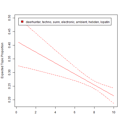
## Topic 1:
##
## Coefficients:
## Estimate Std. Error t value Pr(>|t|)
## (Intercept) 0.417173 0.046938 8.888 < 2e-16 ***
## score -0.020249 0.005925 -3.418 0.000645 ***
## ---
## Signif. codes: 0 '***' 0.001 '**' 0.01 '*' 0.05 '.' 0.1 ' ' 1
##
##
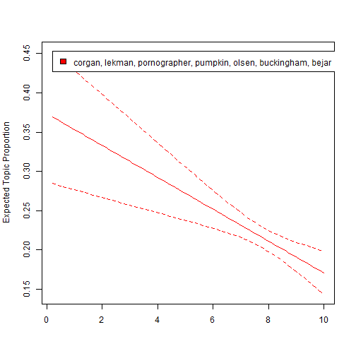
## Topic 2:
##
## Coefficients:
## Estimate Std. Error t value Pr(>|t|)
## (Intercept) 0.373768 0.043059 8.680 < 2e-16 ***
## score -0.020254 0.005477 -3.698 0.000224 ***
## ---
## Signif. codes: 0 '***' 0.001 '**' 0.01 '*' 0.05 '.' 0.1 ' ' 1
##
##
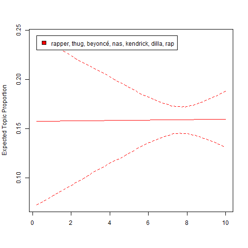
## Topic 3:
##
## Coefficients:
## Estimate Std. Error t value Pr(>|t|)
## (Intercept) 1.588e-01 4.551e-02 3.490 0.000494 ***
## score 5.478e-05 5.788e-03 0.009 0.992449
## ---
## Signif. codes: 0 '***' 0.001 '**' 0.01 '*' 0.05 '.' 0.1 ' ' 1
##
##
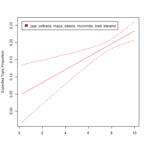
## Topic 4:
##
## Coefficients:
## Estimate Std. Error t value Pr(>|t|)
## (Intercept) 0.045664 0.043347 1.053 0.292262
## score 0.018882 0.005528 3.416 0.000649 ***
## ---
## Signif. codes: 0 '***' 0.001 '**' 0.01 '*' 0.05 '.' 0.1 ' ' 1
##
##
## Topic 5:
##
## Coefficients:
## Estimate Std. Error t value Pr(>|t|)
## (Intercept) 0.005425 0.045205 0.120 0.904482
## score 0.021468 0.005754 3.731 0.000196 ***
## ---
## Signif. codes: 0 '***' 0.001 '**' 0.01 '*' 0.05 '.' 0.1 ' ' 1
plot.estimateEffect(ratingEffect, "score", method = "continuous",
model = topicPredictor, topics = 1, labeltype = "frex")plot.estimateEffect(ratingEffect, "score", method = "continuous",
model = topicPredictor, topics = 2, labeltype = "frex")plot.estimateEffect(ratingEffect, "score", method = "continuous",
model = topicPredictor, topics = 3, labeltype = "frex")plot.estimateEffect(ratingEffect, "score", method = "continuous",
model = topicPredictor, topics = 4, labeltype = "frex")plot.estimateEffect(ratingEffect, "score", method = "continuous",
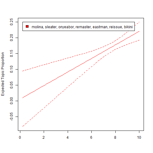
model = topicPredictor, topics = 5, labeltype = "frex")We can see the topic proportion are related to scores for some topics.
From previous visualization, we can see score is an important factor of best new music.
Let's try to use a logistic regression to predict it.
library(DMwR)
library(InformationValue)
library(caret)
set.seed(1234)

sample_set <- sample1 %>%
  pull(.) %>%
  sample.split(SplitRatio = .7)

pfTrain <- subset(sample1, sample_set == TRUE)
pfTest <- subset(sample1, sample_set == FALSE)logit.mod <- glm(best_new_music ~ score, family = "binomial", data = pfTrain)
summary(logit.mod)##
## Call:
## glm(formula = best_new_music ~ score, family = "binomial", data = pfTrain)
##
## Deviance Residuals:
## Min 1Q Median 3Q Max
## -4.1919 -0.1730 -0.0006 0.4381 6.5341
##
## Coefficients:
## Estimate Std. Error z value Pr(>|z|)
## (Intercept) -37.5732 2.2772 -16.50 <2e-16 ***
## score 4.6359 0.2771 16.73 <2e-16 ***
## ---
## Signif. codes: 0 '***' 0.001 '**' 0.01 '*' 0.05 '.' 0.1 ' ' 1
##
## (Dispersion parameter for binomial family taken to be 1)
##
## Null deviance: 1882.53 on 1359 degrees of freedom
## Residual deviance: 658.78 on 1358 degrees of freedom
## AIC: 662.78
##
## Number of Fisher Scoring iterations: 7
logit_pred <- predict(logit.mod, pfTest, type = 'response')
ideal_cutoff <-
  optimalCutoff(
    actuals = pfTest$best_new_music,
    predictedScores = logit_pred,
    optimiseFor = "Both"
  )

logit_pred2 <- ifelse(logit_pred > ideal_cutoff, 1, 0)
logit.matrix <- caret::confusionMatrix(as.factor(logit_pred2), pfTest$best_new_music, positive = "1")
logit.matrix
## Confusion Matrix and Statistics
##
## Reference
## Prediction 0 1
## 0 264 10
## 1 25 284
##
## Accuracy : 0.94
## 95% CI : (0.9175, 0.9578)
## No Information Rate : 0.5043
## P-Value [Acc > NIR] : < 2e-16
##
## Kappa : 0.8799
##
## Mcnemar's Test P-Value : 0.01796
##
## Sensitivity : 0.9660
## Specificity : 0.9135
## Pos Pred Value : 0.9191
## Neg Pred Value : 0.9635
## Prevalence : 0.5043
## Detection Rate : 0.4871
## Detection Prevalence : 0.5300
## Balanced Accuracy : 0.9397
##
## 'Positive' Class : 1
##
Logistic regression achieved 95% accuracy and a kappa of 89.7%.
library(kernlab)

svmTrainControl = trainControl(method = "cv", number = 10, verboseIter = FALSE)

set.seed(1234)
svmPf = train(best_new_music ~ score, data = pfTrain,
  method = "svmLinear", trControl = svmTrainControl,
  tuneGrid = data.frame(C = c(.001, .1, .5, 1, 5, 10, 30)),
  metric = "Accuracy", preProc = c("center", "scale"))

ggplot(svmPf) +
  theme_minimal()
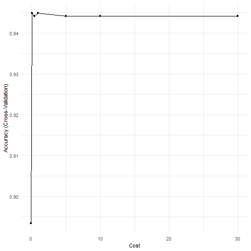
0.1 gives us a really good accuracy.
svmPfTuned = train(best_new_music ~ score, data = pfTrain,
  method = "svmLinear", trControl = svmTrainControl,
  tuneGrid = data.frame(C = 1),
  metric = "Accuracy", preProc = c("center", "scale"))

svmPfTest = predict(svmPfTuned, pfTest)

svmMat <- confusionMatrix(svmPfTest, pfTest$best_new_music,positive = "1")
svmMat
Logistic regression slightly outperforms SVM. (Knitted output is the same as logistic regression somehow. I use a screenshot of Rstudio output here)
In topic modeling, we see some topic thetas are correlated with score. Let's try using thetas and sentiment to predict score.
thetas = topicPredictor$thetasample1_pred <- sample1 %>%
mutate(topic1theta = thetas[,1],
topic2theta = thetas[,2],
topic3theta = thetas[,3],
topic4theta = thetas[,4],
topic5theta = thetas[,5]) %>%
select(-content)set.seed(1234)
sample_set <- sample1_pred %>%
pull(.) %>%
sample.split(SplitRatio = .7)
pfTrain <- subset(sample1_pred, sample_set == TRUE)
pfTest <- subset(sample1_pred, sample_set == FALSE)lmod <- lm(score~sentiment+topic2theta+ topic3theta+topic4theta+topic5theta, data=pfTrain)
summary(lmod)##
## Call:
## lm(formula = score ~ sentiment + topic2theta + topic3theta +
## topic4theta + topic5theta, data = pfTrain)
##
## Residuals:
## Min 1Q Median 3Q Max
## -7.0778 -0.6451 0.2126 0.8071 2.9516
##
## Coefficients:
## Estimate Std. Error t value Pr(>|t|)
## (Intercept) 7.58992 0.09201 82.487 < 2e-16 ***
## sentiment 1.66563 0.39471 4.220 2.61e-05 ***
## topic2theta -1.06255 0.13991 -7.595 5.73e-14 ***
## topic3theta -0.04409 0.14099 -0.313 0.754520
## topic4theta 0.58238 0.15228 3.824 0.000137 ***
## topic5theta 0.93197 0.14594 6.386 2.34e-10 ***
## ---
## Signif. codes: 0 '***' 0.001 '**' 0.01 '*' 0.05 '.' 0.1 ' ' 1
##
## Residual standard error: 1.216 on 1353 degrees of freedom
## Multiple R-squared: 0.1282, Adjusted R-squared: 0.1249
## F-statistic: 39.78 on 5 and 1353 DF, p-value: < 2.2e-16
Even though the linear model does not fit well. We can see sentiment, topic2theta, topic4theta, and topic5theta are significant predictors.

