- Usage, dependencies
- Using a trained model for measuring hypocotyls
- Generating your own training data
- Training a model on your own images
For measuring hypocotyls and training a custom model, it is required to have
- Python >= 3.5
- PyTorch >= 0.4
- NumPy >= 1.13
- Pandas >= 0.23
- scikit-image >= 0.14
- matplotlib >= 3.0
To use the hypocotyl segmentation tool, clone the repository to the local machine:
git clone https://github.com/biomag-lab/hypocotyl-UNetsrc/measure.py can be used for applying the measuring algorithm on custom images, while src/train.py are for training the UNet model on custom annotated data. (Detailed description on them can be found below.)
To apply the algorithm on custom images, the folder containing the images should be organized into the following directory structure:
images_folder
   |-- images
       |-- img001.png
       |-- img002.png
       |-- ...
The src/measure.py script can be used to run the algorithm. The required arguments are
--images_path: path to the images folder, which must have the structure outlined above.--model: path to the UNet model used in the algorithm. Pretrained models are available in themodelsfolder.--result_folder: path to the folder where results will be exported. Additionally, you can specify the following:--device: device to be used for the UNet prediction. Default iscpu, but if a GPU with the CUDA framework installed is available,cuda:$IDcan be used, where$IDis the ID of the GPU. For example,cuda:0. (For PyTorch users: this argument is passed directly to thetorch.Tensor.deviceobject during initialization, which will be used for the rest of the workflow.)--min_object_size: the expected minimum object size in pixels. Default is 50. Detected objects below this size will be filtered out.--max_object_size: the expected maximum object size in pixels. Default isnp.inf. Detected objects above this size will be filtered out.
For instance, an example is the following:
python3 measure.py --images_path path_to_images \
    --model ../models/unet \
    --result_folder path_to_results \
--device cuda:0In case the algorithm performs poorly, for instance if the images were taken under very different conditions than the ones provided to the available model during training, the UNet backbone model can be retrained on custom data. This process is called annotation, which can be done easily with ImageJ.
Step 1. Organize your images to be annotated such that each image is contained in a separate folder with common root. The folder should be named after the image. For example:
images_folder
   |-- image_1
       |-- image_1.png
   |-- image_2
       |-- image_2.png
   |-- ...
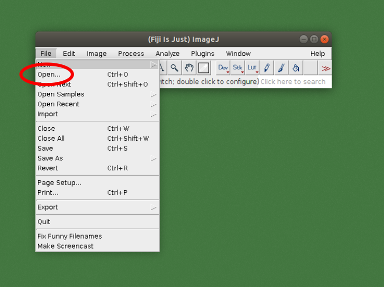
Step 2. Open the image to be annotated in ImageJ.
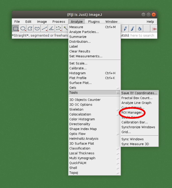
Step 3. Open the ROI manager tool.
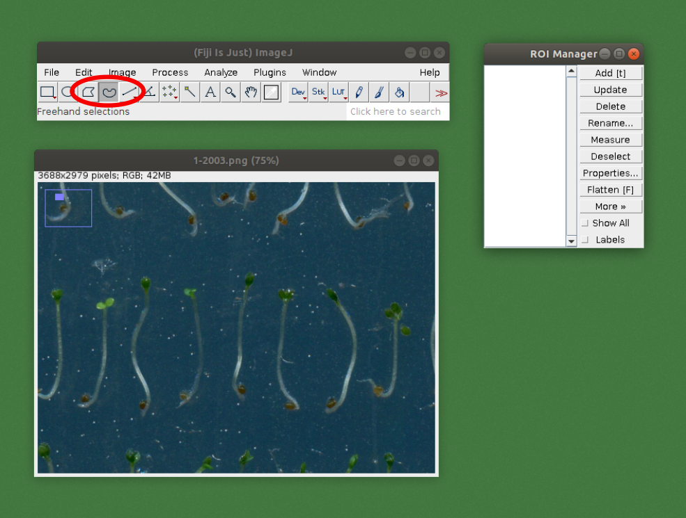
Step 4. Select an appropriate selection tool, for example Freehand selections.
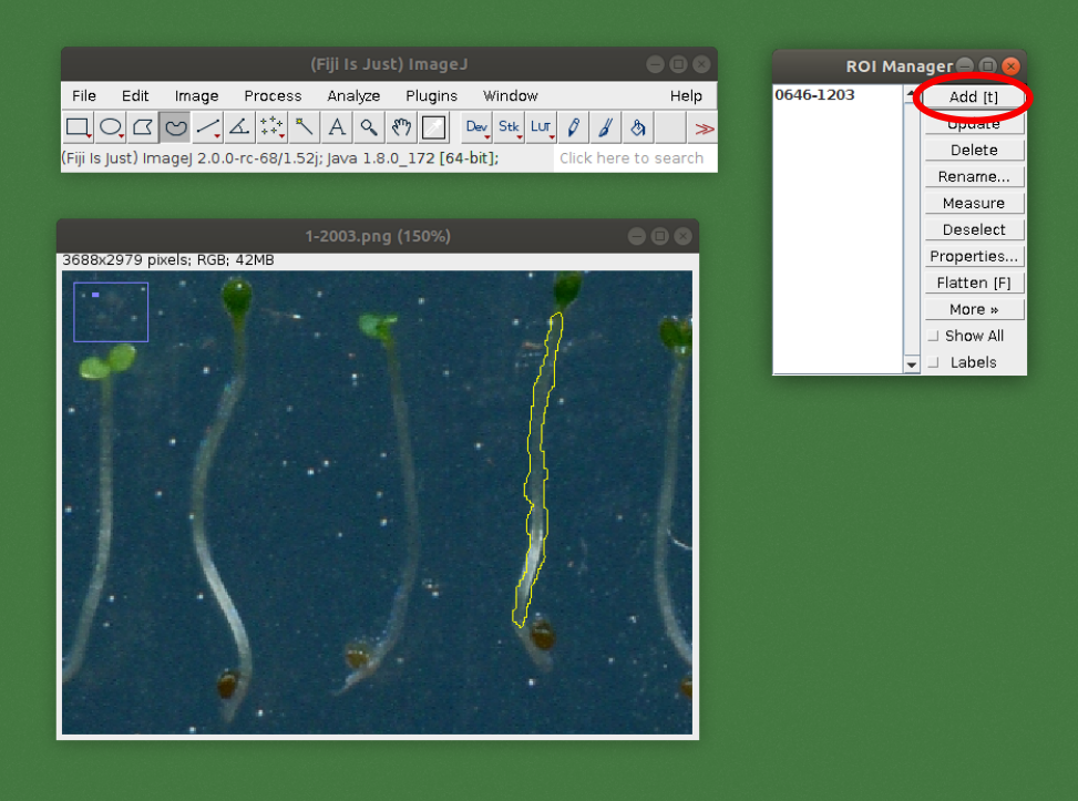
Step 5. Draw the outline of the part which is part of the plant and should be included during the measurements. Press t or click on the Add [t] button to add the selected part to the ROI manager.
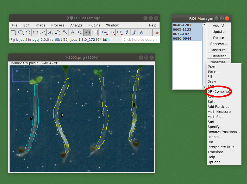
Step 6. Repeat the outlining with all of the selections, adding them one by one. When it is done, select all and click More > OR (Combine).
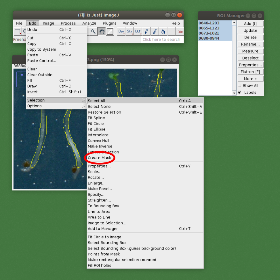
Step 7. Press Edit > Selection > Create Mask. This will open up a new image.
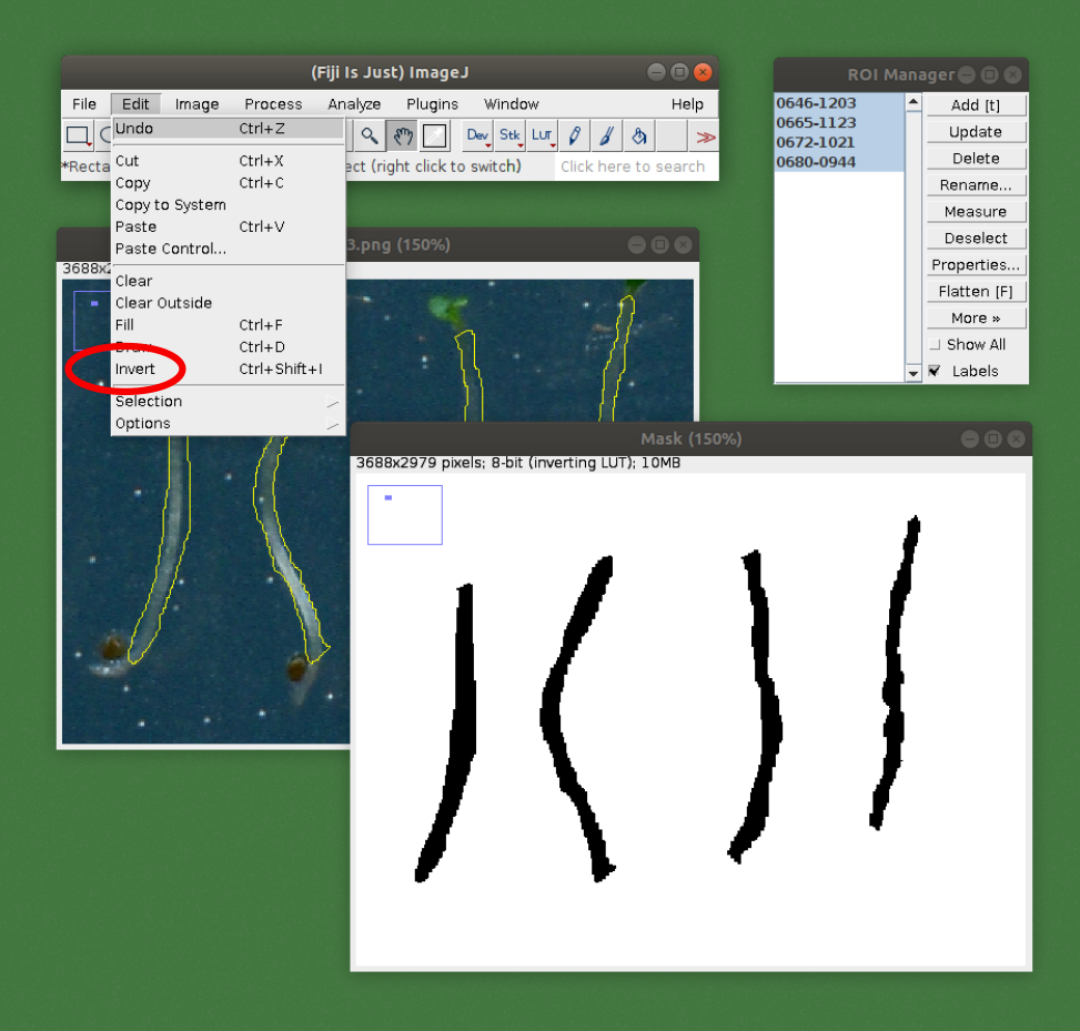
Step 8. Invert the mask image by pressing Edit > Invert or pressing Ctrl + Shift + I.
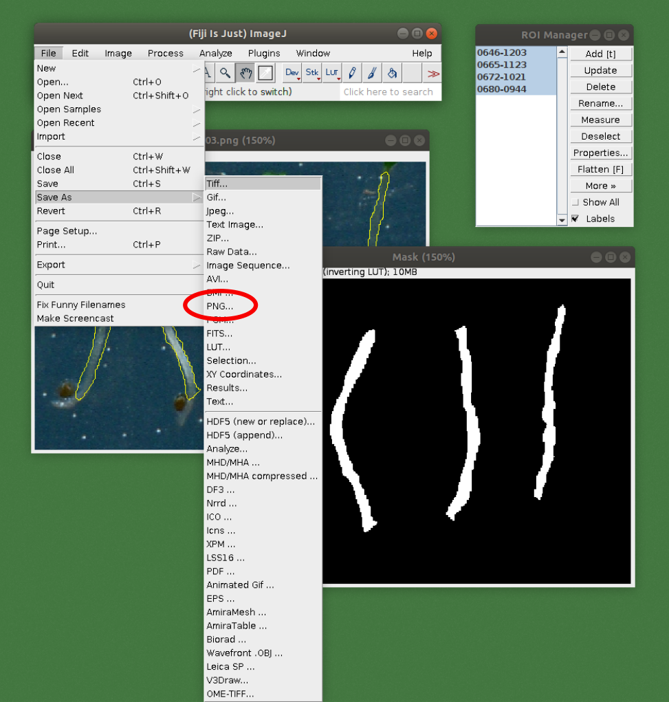
Step 9. Save the mask image to the folder with the original. Add the suffix -hypo to the name. For example, if the original name was image_1.png, this image should be named image_1-hypo.png.
Step 10. Repeat the same process to annotate the parts of the plant which should not be included in the measurements. Save the mask to the same folder. Add the suffix -nonhypo to the name.
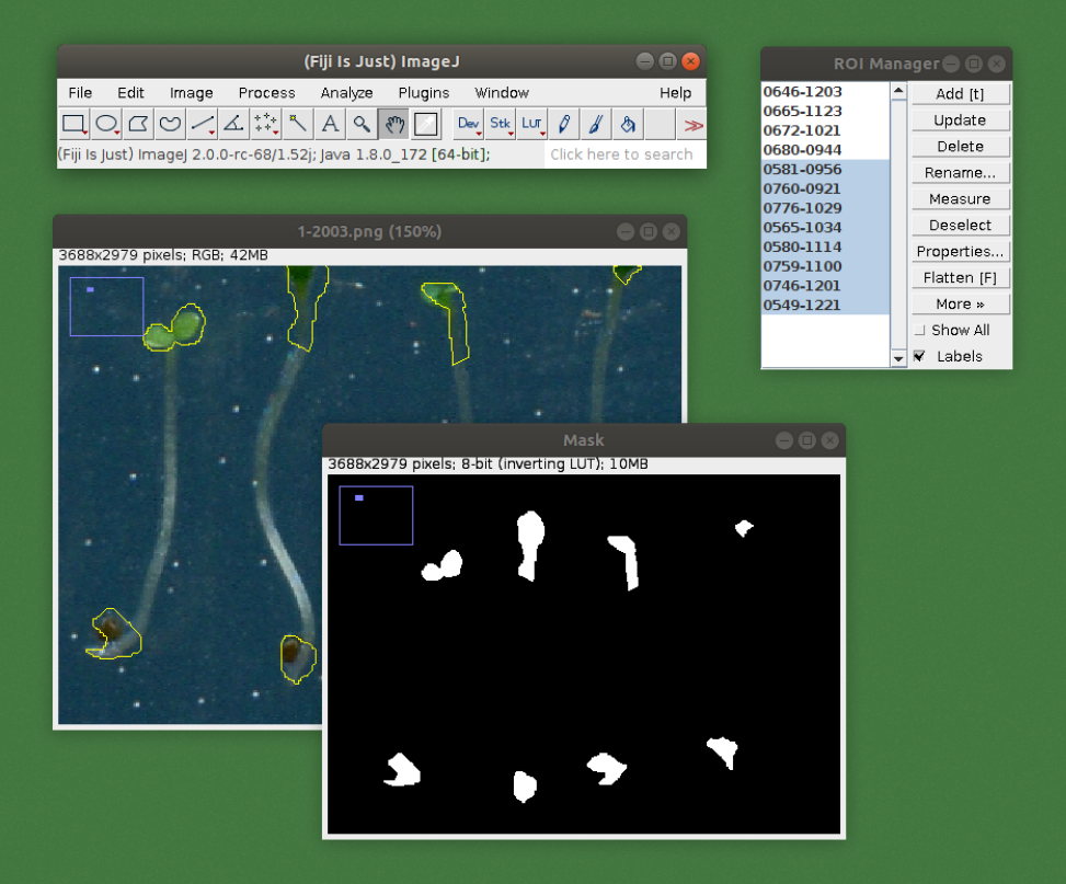
Step 11. Create the training data for the algorithm by running the src/preprocessing/mask.py. The required arguments are
--images_folder: path to the folder where the folders containing the images and masks located.--export_folder: path to the folder where the results should be exported.--make_patches: True if images and masks are to be patched up to smaller pieces. Recommended for training.
If custom annotated data is available, the containing folder should be organized into the following directory structure:
images_folder
   |-- images
       |-- img001.png
       |-- img002.png
       |-- ...
   |-- masks
       |-- img001.png
       |-- img002.png
       |-- ...
The mask images should have identical name to their corresponding image. After the training data is organized, the src/train.py script can be used to train a custom UNet model. The required arguments are
--train_dataset: path to the folder where the training data is located. This should match with the--export_folderargument given to thesrc/preprocessing/mask.pyscript during Step 11. of the previous point.
The optional arguments are
--epochs: the number of epochs during training. Default is 1000, but this is very dependent on the dataset and data augmentation method used.--batch_size: the size of the batch during training. Default is 1. If GPU is used, it is recommended to select batch size as large as GPU memory allows.--initial_lr: initial learning rate. Default is 1e-3, which proved to be the best for the training dataset used. (Different datasets might have more optimal initial learning rates.)--model_name: name of the model. Default is UNet-hypocotyl.--trained_model_path: to continue training of a previously trained model, its path can be given.--val_dataset: path to the folder where the validation data is located. During training, validation data is used to catch overfitting and apply early stopping.--model_save_freq: frequency of model saving. Default is 200, which means that the model is saved after every 200th epoch.--device: device to be used for the UNet training. Default iscpu, but if a GPU with the CUDA framework installed is available,cuda:$IDcan be used, where$IDis the ID of the GPU. For example,cuda:0. (For PyTorch users: this argument is passed directly to thetorch.Tensor.deviceobject during initialization, which will be used for the rest of the workflow.)