The goals / steps of this project are the following:
- Perform a Histogram of Oriented Gradients (HOG) feature extraction on a labeled training set of images and train a classifier Linear SVM classifier
- Optionally, you can also apply a color transform and append binned color features, as well as histograms of color, to your HOG feature vector.
- Note: for those first two steps don't forget to normalize your features and randomize a selection for training and testing.
- Implement a sliding-window technique and use your trained classifier to search for vehicles in images.
- Run your pipeline on a video stream (start with the test_video.mp4 and later implement on full project_video.mp4) and create a heat map of recurring detections frame by frame to reject outliers and follow detected vehicles.
- Estimate a bounding box for vehicles detected.
Link to YouTube Video: https://youtu.be/gVmqyGoVTgw
Rubric Points
Here I will consider the rubric points individually and describe how I addressed each point in my implementation.
All code can be found in the IPython Notebook at this directory: ./vehicle_detection.ipynb.
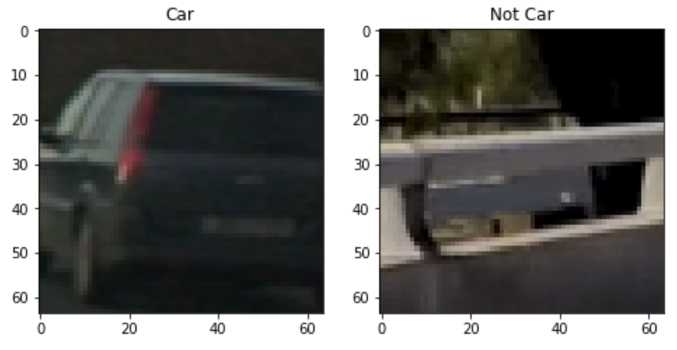
First, the vehicle and non-vehicle data was read into the variables cars and not_cars in cell 8. Visuals of cars and not_cars were displayed in cell 9 as follows:
I then explored different color spaces and different skimage.hog() parameters (orientations, pixels_per_cell, and cells_per_block). I used the test images to visualize the cars in the image and the areas around the car to see which color space would be most effective.
Here are examples of the various color spaces:
-
HOG (Histogram of Oriented Gradients):
- cells_per_block
- pixels_per_cell
- orientations
- channel
-
Color Histogram:
- The number of histogram bins.
-
Spacial Bin (features from pixels):
- color_space
- spacial_size
The HOG parameters were chosen based on the SVM model accuracy, performance, and trial an error through visualizing the final output of vehicle positions.
In order to reduce the vector length a spatial_size of (16, 16) was chosen which would allow for better performance. hist_feat were set to False as the accuracy gain over performance was not significant. This also applied to hog_channel. In increase both performance and accuracy when detecting vehicles, only a portion of the image was used when the sliding window function was applied. This reduced the number of false positives and increased performance by removing redundant/ unnecessary window searches.
In cell 13 parameter tuning was performed using the from sklearn.model_selection import GridSearchCV. This allowed for the C parameter to be tuned and to determine if a Linear or RBF model would be best suited for detecting vehicles.
Based on these results, a RBF model was chosen with a C value of 10.
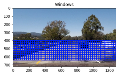
Sliding window functions were implemented in cell 4.
These values were determined by trial an error and visualizing the final output of the model. Various parameter combinations were used. While some parameters of certain values provided better accuracy, is significantly reduced the performance of the model. One in particular was the window size. A bigger window size of (96, 96) performed better than a model using a window size of (32, 32). A window size of (96, 96) also allowed vehicles to be detected which were closer and considered more important that vehicles further away.
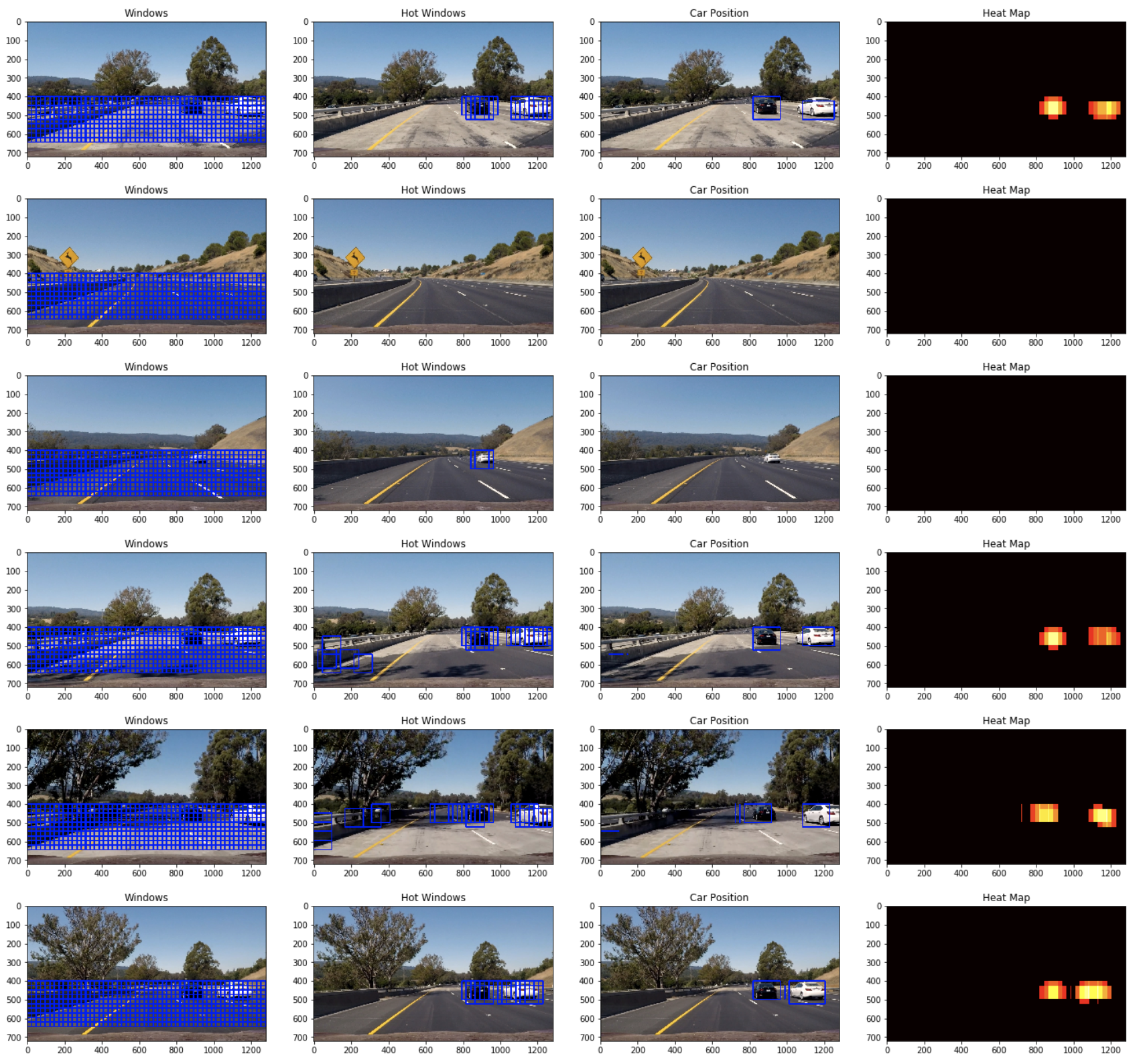
To optimize performance, a spatial_size of (16, 16) was used to reduce the number of feature vectors. Furthermore hist_feat was set to False as the accuracy gain over performance was not significant. Here are some examples:
Here's a link to my video result
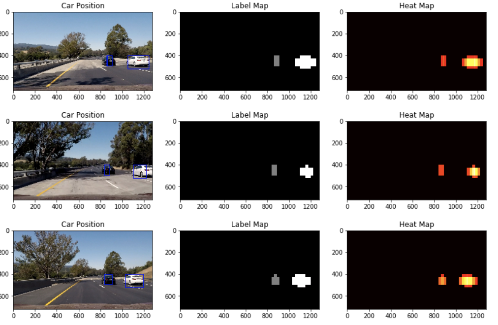
I recorded the positions of positive detections in each frame of the video. From the positive detections I created a heatmap and then thresholded that map to identify vehicle positions. I then used scipy.ndimage.measurements.label() to identify individual blobs in the heatmap. I then assumed each blob corresponded to a vehicle. I constructed bounding boxes to cover the area of each blob detected.
Here's an example result showing the heatmap from a series of frames of video, the result of scipy.ndimage.measurements.label() and the bounding boxes then overlaid on the last frame of video:
1. Issues faced during the implementation of the pipeline and where it is likely to fail. What could be improved to make it more robust?to make it more robust?
In my pipeline, it displayed false positives when there were shadows or darker areas. This could potentially be corrected by lightening images as they are passed into the pipeline or implement shadow removal. The implementation also struggled to identify the correct bounding area for the car as in some cased the box did not surround the entire car. The implementation also cannot be run in real time as it has not been optimized enough.


