This repository contains code (training / metrics / plotting) to investigate disentangling in VAE as well as compare 5 different losses (summary of the differences) using a single architecture:
- Standard VAE Loss from Auto-Encoding Variational Bayes
- β-VAEH from β-VAE: Learning Basic Visual Concepts with a Constrained Variational Framework
- β-VAEB from Understanding disentangling in β-VAE
- FactorVAE from Disentangling by Factorising
- β-TCVAE from Isolating Sources of Disentanglement in Variational Autoencoders
Notes:
- Tested for python >= 3.6
- Tested for CPU and GPU
Table of Contents:
# clone repo
pip install -r requirements.txt
Use python main.py <model-name> <param> to train and/or evaluate a model. For example:
python main.py btcvae_celeba_mini -d celeba -l btcvae --lr 0.001 -b 256 -e 5
You can run predefined experiments and hyper-parameters using -x <experiment>. Those hyperparameters are found in hyperparam.ini. Pretrained models for each experiment can be found in results/<experiment> (created using ./bin/train_all.sh).
This will create a directory results/<saving-name>/ which will contain:
- model.pt: The model at the end of training.
- model-
i.pt: Model checkpoint afteriiterations. By default saves every 10. - specs.json: The parameters used to run the program (default and modified with CLI).
- training.gif: GIF of latent traversals of the latent dimensions Z at every epoch of training.
- train_losses.log: All (sub-)losses computed during training.
- test_losses.log: All (sub-)losses computed at the end of training with the model in evaluate mode (no sampling).
- metrics.log: Mutual Information Gap metric and Axis Alignment Metric. Only if
--is-metric(slow).
usage: main.py ...

PyTorch implementation and evaluation of disentangled Variational AutoEncoders
and metrics.

optional arguments:
  -h, --help            show this help message and exit

General options:
  name                  Name of the model for storing or loading purposes.
  -L, --log-level {CRITICAL,ERROR,WARNING,INFO,DEBUG,NOTSET}
                        Logging levels. (default: info)
  --no-progress-bar     Disables progress bar. (default: False)
  --no-cuda             Disables CUDA training, even when have one. (default:
                        False)
  -s, --seed SEED       Random seed. Can be `None` for stochastic behavior.
                        (default: 1234)

Training specific options:
  --checkpoint-every CHECKPOINT_EVERY
                        Save a checkpoint of the trained model every n epoch.
                        (default: 30)
  -d, --dataset {mnist,fashion,dsprites,celeba,chairs}
                        Path to training data. (default: mnist)
  -x, --experiment {custom,debug,best_celeba,VAE_mnist,VAE_fashion,VAE_dsprites,VAE_celeba,VAE_chairs,betaH_mnist,betaH_fashion,betaH_dsprites,betaH_celeba,betaH_chairs,betaB_mnist,betaB_fashion,betaB_dsprites,betaB_celeba,betaB_chairs,factor_mnist,factor_fashion,factor_dsprites,factor_celeba,factor_chairs,btcvae_mnist,btcvae_fashion,btcvae_dsprites,btcvae_celeba,btcvae_chairs}
                        Predefined experiments to run. If not `custom` this
                        will overwrite some other arguments. (default: custom)
  -e, --epochs EPOCHS   Maximum number of epochs to run for. (default: 100)
  -b, --batch-size BATCH_SIZE
                        Batch size for training. (default: 64)
  --lr LR               Learning rate. (default: 0.0005)

Model specfic options:
  -m, --model-type {Burgess}
                        Type of encoder and decoder to use. (default: Burgess)
  -z, --latent-dim LATENT_DIM
                        Dimension of the latent variable. (default: 10)
  -l, --loss {VAE,betaH,betaB,factor,btcvae}
                        Type of VAE loss function to use. (default: betaB)
  -r, --rec-dist {bernoulli,laplace,gaussian}
                        Form of the likelihood ot use for each pixel.
                        (default: bernoulli)
  -a, --reg-anneal REG_ANNEAL
                        Number of annealing steps where gradually adding the
                        regularisation. What is annealed is specific to each
                        loss. (default: 0)

BetaH specific parameters:
  --betaH-B BETAH_B     Weight of the KL (beta in the paper). (default: 4)

BetaB specific parameters:
  --betaB-initC BETAB_INITC
                        Starting annealed capacity. (default: 0)
  --betaB-finC BETAB_FINC
                        Final annealed capacity. (default: 25)
  --betaB-G BETAB_G     Weight of the KL divergence term (gamma in the paper).
                        (default: 1000)

factor VAE specific parameters:
  --factor-G FACTOR_G   Weight of the TC term (gamma in the paper). (default:
                        6)
  --lr-disc LR_DISC     Learning rate of the discriminator. (default: 5e-05)

beta-tcvae specific parameters:
  --btcvae-A BTCVAE_A   Weight of the MI term (alpha in the paper). (default:
                        1)
  --btcvae-G BTCVAE_G   Weight of the dim-wise KL term (gamma in the paper).
                        (default: 1)
  --btcvae-B BTCVAE_B   Weight of the TC term (beta in the paper). (default:
                        6)

Evaluation specific options:
  --is-eval-only        Whether to only evaluate using precomputed model
                        `name`. (default: False)
  --is-metrics          Whether to compute the disentangled metrcics.
                        Currently only possible with `dsprites` as it is the
                        only dataset with known true factors of variations.
                        (default: False)
  --no-test             Whether not to compute the test losses.` (default:
                        False)
  --eval-batchsize EVAL_BATCHSIZE
                        Batch size for evaluation. (default: 1000)
Use python main_viz.py <model-name> <plot_types> <param> to plot using pretrained models. For example:
python main_viz.py btcvae_celeba_mini gif-traversals reconstruct-
                        traverse -c 7 -r 6 -t 2 --is-posterior
This will save the plots in the model directory results/<model-name>/. Generated plots for all experiments are found in their respective directories (created using ./bin/plot_all.sh).
usage: main_viz.py ...

CLI for plotting using pretrained models of `disvae`

positional arguments:
  name                  Name of the model for storing and loading purposes.
  {generate-samples,data-samples,reconstruct,traversals,reconstruct-traverse,gif-traversals,all}
                        List of all plots to generate. `generate-samples`:
                        random decoded samples. `data-samples` samples from
                        the dataset. `reconstruct` first rnows//2 will be the
                        original and rest will be the corresponding
                        reconstructions. `traversals` traverses the most
                        important rnows dimensions with ncols different
                        samples from the prior or posterior. `reconstruct-
                        traverse` first row for original, second are
                        reconstructions, rest are traversals. `gif-traversals`
                        grid of gifs where rows are latent dimensions, columns
                        are examples, each gif shows posterior traversals.
                        `all` runs every plot.

optional arguments:
  -h, --help            show this help message and exit
  -s, --seed SEED       Random seed. Can be `None` for stochastic behavior.
                        (default: None)
  -r, --n-rows N_ROWS   The number of rows to visualize (if applicable).
                        (default: 6)
  -c, --n-cols N_COLS   The number of columns to visualize (if applicable).
                        (default: 7)
  -t, --max-traversal MAX_TRAVERSAL
                        The maximum displacement induced by a latent
                        traversal. Symmetrical traversals are assumed. If
                        `m>=0.5` then uses absolute value traversal, if
                        `m<0.5` uses a percentage of the distribution
                        (quantile). E.g. for the prior the distribution is a
                        standard normal so `m=0.45` corresponds to an absolute
                        value of `1.645` because `2m=90%` of a standard normal
                        is between `-1.645` and `1.645`. Note in the case of
                        the posterior, the distribution is not standard normal
                        anymore. (default: 2)
  -i, --idcs IDCS [IDCS ...]
                        List of indices to of images to put at the begining of
                        the samples. (default: [])
  -u, --upsample-factor UPSAMPLE_FACTOR
                        The scale factor with which to upsample the image (if
                        applicable). (default: 1)
  --is-show-loss        Displays the loss on the figures (if applicable).
                        (default: False)
  --is-posterior        Traverses the posterior instead of the prior.
                        (default: False)
Here are examples of plots you can generate:
-
python main_viz.py <model> reconstruct-traverse --is-show-loss --is-posteriorfirst row are originals, second are reconstructions, rest are traversals. Shown forbtcvae_dsprites: -
python main_viz.py <model> gif-traversalsgrid of gifs where rows are latent dimensions, columns are examples, each gif shows posterior traversals. Shown forbtcvae_celeba: -
Grid of gifs generated using code in
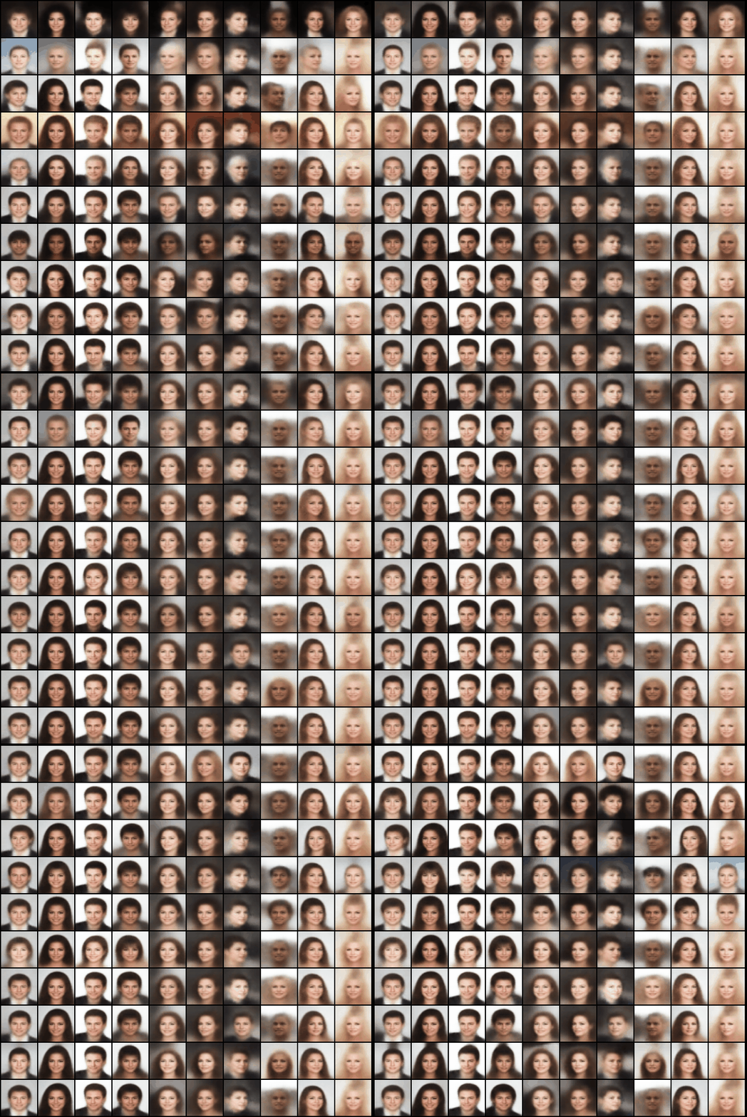
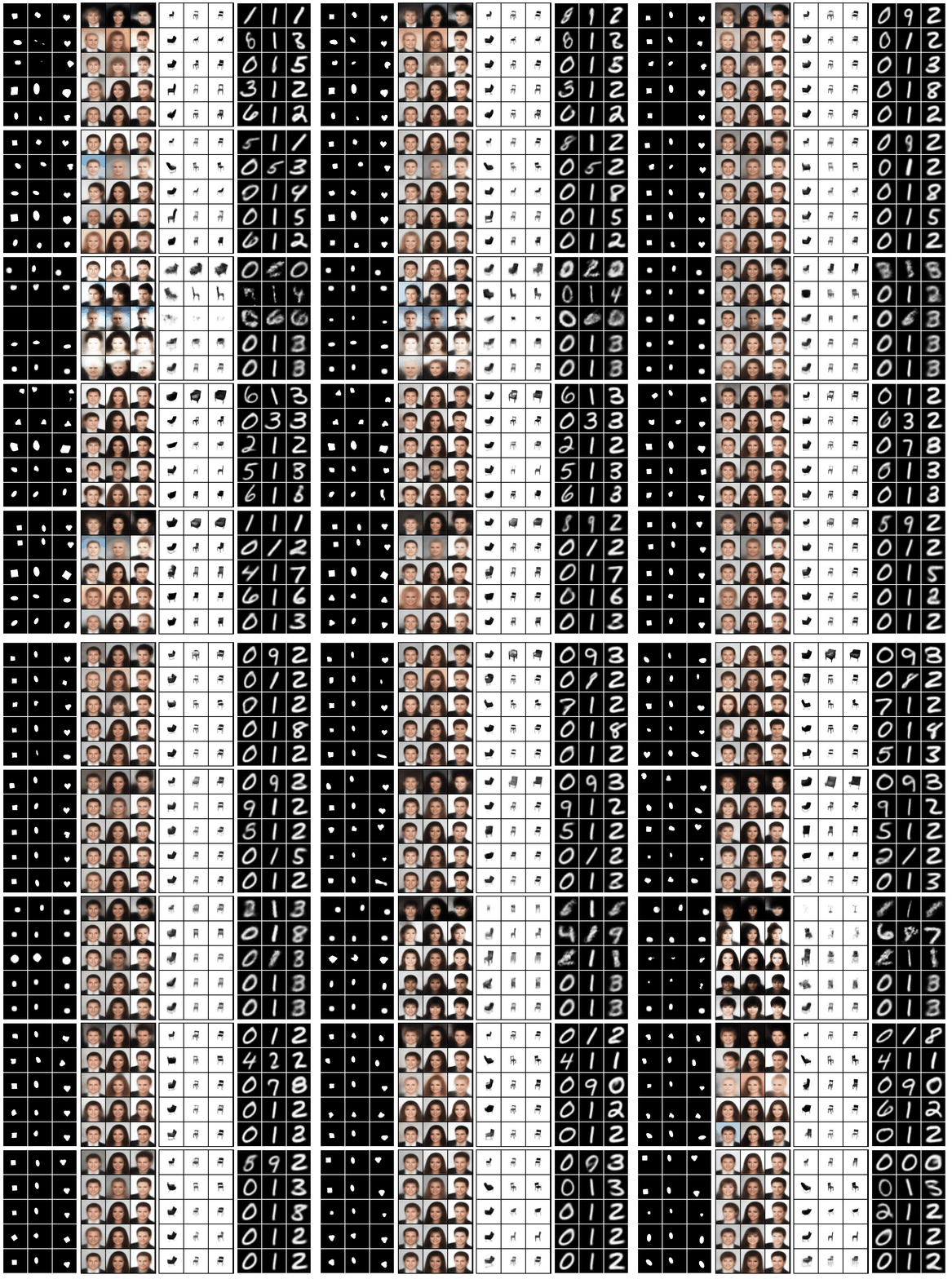
bin/plot_all.sh. The columns of the grid correspond to the datasets (besides FashionMNIST), the rows correspond to the models (in order: Standard VAE, β-VAEH, β-VAEB, FactorVAE, β-TCVAE):
For more examples, all of the plots for the predefined experiments are found in their respective directories (created using ./bin/plot_all.sh).
Current datasets that can be used:
The dataset will be downloaded the first time you run it and will be stored in data for future uses. The download will take time and might not work anymore if the download links change. In this case either:
- Open an issue
- Change the URLs (
urls["train"]) for the dataset you want inutils/datasets.py(please open a PR in this case :) ) - Download by hand the data and save it with the same names (not recommended)
In addition to replicating the aforementioned papers, we also propose and investigate the following:
Qualitative inspections are unsuitable to compare models reliably due to their subjective and time consuming nature. Recent papers use quantitative measures of disentanglement based on the ground truth factors of variation v and the latent dimensions z. The Mutual Information Gap (MIG) metric is an appealing information theoretic metric which is appealing as it does not use any classifier. To get a MIG of 1 in the dSprites case where we have 10 latent dimensions and 5 generative factors, 5 of the latent dimensions should exactly encode the true factors of variations, and the rest should be independent of these 5.
Although a metric like MIG is what we would like to use in the long term, current models do not get good scores and it is hard to understand what they should improve. We thus propose an axis alignment metric AAM, which does not focus on how much information of v is encoded by z, but rather if each vk is only encoded in a single zj. For example in the dSprites dataset, it is possible to get an AAM of 1 if z encodes only 90% of the variance in the x position of the shapes as long as this 90% is only encoded by a single latent dimension zj. This is a useful metric to have a better understanding of what each model is good and bad at. Formally:
Where the subscript (d) denotes the dth order statistic and Ix is estimated using empirical distributions and stratified sampling (like with MIG):
The model is decoupled from all the losses and it should thus be very easy to modify the encoder / decoder without modifying the losses. We only used a single model in order to have more objective comparisons of the different losses. The model used is the one from Understanding disentangling in β-VAE, which is summarized below:
All the previous losses are special cases of the following loss:
-
Index-code mutual information: the mutual information between the latent variables z and the data variable x. There is contention in the literature regarding the correct way to treat this term. From the information bottleneck perspective this should be penalized. InfoGAN get good results by increasing the mutual information (negative α). Finally, Wasserstein Auto-Encoders drops this term.
-
Total Correlation (TC): the KL divergence between the joint and the product of the marginals of the latent variable. I.e.* a measure of dependence between the latent dimensions. Increasing β forces the model to find statistically independent factors of variation in the data distribution.
-
Dimension-wise KL divergence: the KL divergence between each dimension of the marginal posterior and the prior. This term ensures the learning of a compact space close to the prior which enables sampling of novel examples.
The losses differ in their estimates of each of these terms and the hyperparameters they use:
- Standard VAE Loss: α=β=ɣ=1. Each term is computed exactly by a closed form solution (KL between the prior and the posterior). Tightest lower bound.
- β-VAEH: α=β=ɣ>1. Each term is computed exactly by a closed form solution. Simply adds a hyper-parameter (β in the paper) before the KL.
- β-VAEB: α=β=ɣ>1. Same as β-VAEH but only penalizes the 3 terms once they deviate from a capacity C which increases during training.
- FactorVAE: α=ɣ=1, β>1. Each term is computed exactly by a closed form solution. Simply adds a hyper-parameter (β in the paper) before the KL. Adds a weighted Total Correlation term to the standard VAE loss. The total correlation is estimated using a classifier and the density-ratio trick. Note that ɣ in their paper corresponds to β+1 in our framework.
- β-TCVAE: α=ɣ=1 (although can be modified), β>1. Conceptually equivalent to FactorVAE, but each term is estimated separately using minibatch stratified sampling.
When using one of the models implemented in this repo in academic work please cite the corresponding paper (linked at the top of the README). In case you want to cite this specific implementation then you can use:
@misc{dubois2019dvae,
  title        = {Disentangling VAE},
  author       = {Dubois, Yann and Kastanos, Alexandros and Lines, Dave and Melman, Bart},
  month        = {march},
  year         = {2019},
  howpublished = {\url{http://github.com/YannDubs/disentangling-vae/}}
}


