This is the code related to the paper "Benchmarks and Custom Package for Electrical Load Forecasting". This repository mainly aims at implementing routines for probabilistic energy forecasting. However, we also provide the implementation of relevant point forecasting models. The datasets and their forecasting results in this archive are transferring to an anonymous shared document. To reproduce the results in our archive, users can refer to the process in the main.py file. Users can easily construct different forecasting models by selecting different Feature engineering methods and preprocessing, post-processing, and training models.
We include several different datasets in our load forecasting archive. And there is the summary of them.
| Dataset | No.of series | Length | Resolution | Load type | External variables | |
|---|---|---|---|---|---|---|
| 1 | Covid19 | 1 | 31912 | hourly | aggregated | airTemperature, Humidity, etc |
| 2 | GEF12 | 20 | 39414 | hourly | aggregated | airTemperature |
| 3 | GEF14 | 1 | 17520 | hourly | aggregated | airTemperature |
| 4 | GEF17 | 8 | 17544 | hourly | aggregated | airTemperature |
| 5 | PDB | 1 | 17520 | hourly | aggregated | airTemperature |
| 6 | Spanish | 1 | 35064 | hourly | aggregated | airTemperature, seaLvlPressure, etc |
| 7 | Hog | 24 | 17544 | hourly | building | airTemperature, wind speed, etc |
| 8 | Bull | 41 | 17544 | hourly | building | airTemperature, wind speed, etc |
| 9 | Cockatoo | 1 | 17544 | hourly | building | airTemperature, wind speed, etc |
| 10 | ELF | 1 | 21792 | hourly | aggregated | No |
| 11 | UCI | 321 | 26304 | hourly | building | No |
- Python
- Conda
This is only needed when used the first time on the machine.
conda env create --file proenfo_env.ymlconda activate proenfo_env
conda deactivateIf there's a new package in the proenfo_env.yml file you have to update the packages in your local env
conda env update -f proenfo_env.ymlExport your environment for other users
conda env export > proenfo_env.yml conda env remove --name proenfo_env
conda env create --file proenfo_env.yml- python=3.9.13
- numpy
- pandas
- scikit-learn
- matplotlib
- plotly
- statsmodels
- xlrd
- jupyterlab
- nodejs
- mypy
- pytorch
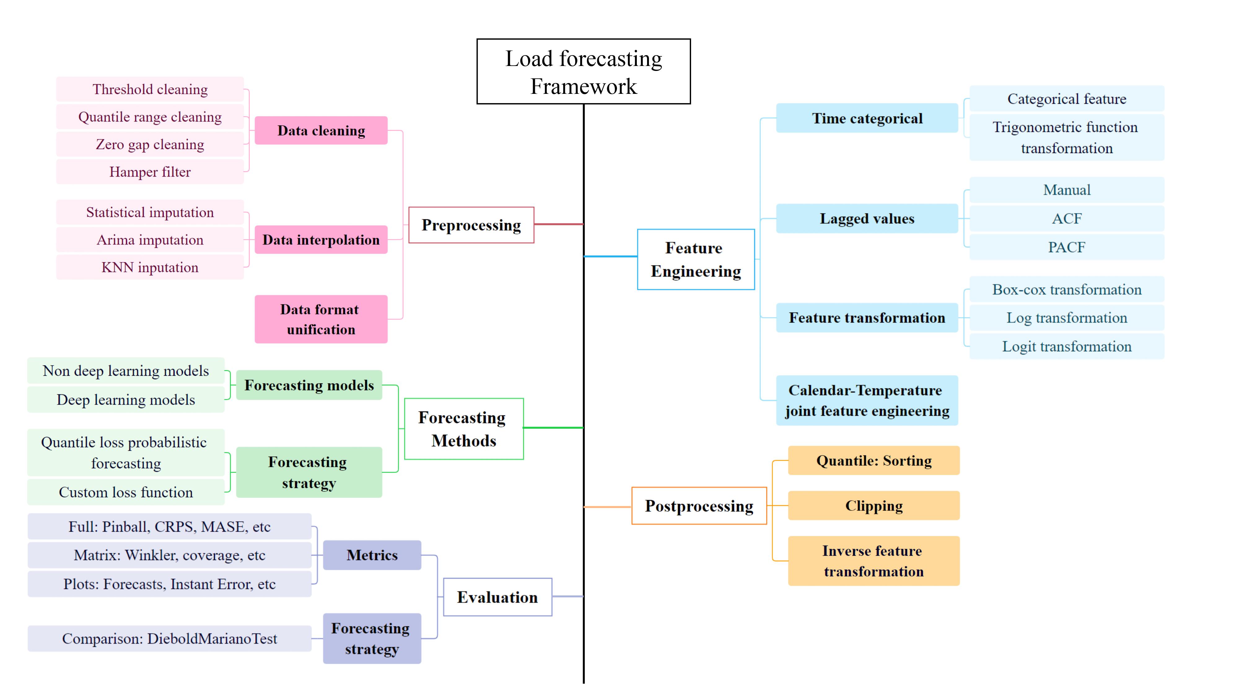
Our package covers the entire process of constructing forecasting models, including data preprocessing, construction of forecasting models, etc.
| Models | Paper | Type | Description | |
|---|---|---|---|---|
| 1 | BMQ | Non-deep learning | moving quantity method based on a fixed number of past time points | |
| 2 | BEQ | Non-deep learning | moving quantity method based on all historical data | |
| 3 | BCEP | Non-deep learning | take the forecasting error obtained by the persistence method as quantile forecasting | |
| 4 | QCE | Non-deep learning | take the forecasting error obtained by the linear regression as quantile forecasting | |
| 5 | KNNR | link | Non-deep learning | quantile regression based on K-nearest neighbor |
| 6 | RFR | link | Non-deep learning | quantile regression based on random forest |
| 7 | SRFR | link | Non-deep learning | quantile regression based on sample random forest |
| 8 | ERT | link | Non-deep learning | quantile regression based on extreme random tree |
| 9 | SERT | link | Non-deep learning | quantile regression based on sample extreme random tree |
| 10 | FFNN | link | deep learning | quantile regression based on feed-forward neural network |
| 11 | LSTM | link | deep learning | quantile regression based on LSTM |
| 12 | CNN | link | deep learning | quantile regression based on CNN |
| 13 | Transformer | link | deep learning | quantile regression based on Transformer |
| 14 | LSTNet | link | deep learning | quantile regression based on LSTNet |
| 15 | Wavenet | link | deep learning | quantile regression based on Wavenet |
| 16 | N-BEATS | link | deep learning | quantile regression based on N-BEATS |
| 17 | DLinear | deep learning | quantile regression based on DLinear | |
| 18 | NLinear | deep learning | quantile regression based on NLinear | |
| 19 | Autoformer | deep learning | quantile regression based on Autoformer | |
| 20 | Fedformer | deep learning | quantile regression based on Fedformer | |
| 21 | Informer | deep learning | quantile regression based on Informer |
To start forecasting, we first need to import some packages.
import datetime as dt
import os
import pandas as pd
import evaluation.metrics as em
import feature.feature_lag_selection as fls
import feature.feature_external_selection as fes
import feature.feature_transformation as ft
import feature.time_categorical as tc
import feature.time_stationarization as ts
import models.model_init as mi
import models.benchmark_init as bi
import postprocessing.quantile as ppq
import postprocessing.value as ppv
from forecast.scenario import calculate_scenario
import random
import torch
import pickle
import argparse
import numpy as np
import warnings
warnings.filterwarnings("ignore")
import ast
Import the dataset, the example of the format of the dataset can be seen in ./data.
site_id = 'GFC14_load'
file_name = "load_with_weather.pkl"
data = pd.read_pickle(f"data/{site_id}/{file_name}")
target = 'load'
Define your forecasting setting, eg, forecasting quantiles, and feature engineering strategy.
err_tot, forecast_tot, true = calculate_scenario(data=data,
                                                target=target,
                                                methods_to_train=methods_to_train,
                                                horizon=horizon,
                                                train_ratio=train_ratio,
                                                feature_transformation=feature_transformation,
                                                time_stationarization=time_stationarization,
                                                datetime_features=datetime_features,
                                                target_lag_selection=target_lag_selection,
                                                external_feature_selection=external_feature_selection,
                                                post_processing_quantile=post_processing_quantile,
                                                post_processing_value=post_processing_value,
                                                evaluation_metrics=evaluation_metrics,
                                                device = device,
                                                prob_forecasting = False,
                                                strategy=train_stratehy,
                                                data_name=name
                                                            )
from scipy.io import loadmat
breakpoint_new=loadmat('./simulated_data/breakpoint_new.mat')
breakpoint_new.pop("__header__")
breakpoint_new.pop("__version__")
breakpoint_new.pop("__globals__")
breakpoint_raw=list(breakpoint_new.values())
breakpoint = pytorchtools.breakpoint_generator(breakpoint_raw)[8]#take hour 9 as an example
loss_function = pytorchtools.ContinuousPiecewiseLinearFunction(breakpoint)Based on Pytorch, users can simply add their own defined deep learning network to our forecasting framework. Firstly, users need to define the initialization method for the model in ./models/model_init.py
class MYQuantile_Regressor(MultiQuantileRegressor):
    def __init__(self, quantiles: List[float] = [0.1,0.2,0.3,0.4,0.5,0.6,0.7,0.8,0.9]):
        super().__init__(
            X_scaler=StandardScaler(),
            y_scaler=StandardScaler(),
            quantiles=quantiles)

    def set_params(self, input_dim: int,external_features_diminsion: int):
        self.model = models.pytorch.PytorchRegressor(
            model=models.pytorch.MYQuantile_Model(input_dim,external_features_diminsion, n_output=len(self.quantiles)),
            loss_function=pytorchtools.PinballLoss(self.quantiles))
        return self
Secondly, users need to add the structure of the model in ./models/pytorch.py
class MYQuantile_Model(nn.Module):
    def __init__(self,input_parameters):
        super(MYQuantile_Model, self).__init__()
        '''
        build your model here
        '''
    def forward(self, X_batch,X_batch_ex):
        '''
        input the data into the model, here X_batch is the sequence data while X_batch_ex is the external variable.
        '''
        return output
Finally, you can add your model to the methods_to_train.
methods_to_train.append(mi.MYQuantile_Regressor())We include several metrics to evaluate the forecasting performance and summarize them below. For details, users can check it in ./evaluation/metrics.py
| Metrics | Calculation method | Metric type | Description | |
|---|---|---|---|---|
| 1 | CoverageError (CE) | probility | measures the difference between the proportion of actual observations falling within the forecasting interval and the expected coverage rate | |
| 2 | Winkler Score (WS) | - | probability | evaluates whether the forecasting interval accurately captures actual observations, taking into account the width of the interval. |
| 3 | Pinball Loss (PL) | probability | weights the error based on whether the forecasting value falls on the side of the actual observation value (above or below) | |
| 4 | RampScore (RS) | - | probability | measures the consistency of the slope (i.e. increasing or decreasing trend) |
| 5 | CalibrationError | - | probability | evaluates the accuracy of forecasting models in representing uncertainty |
| 6 | IntervalWidth | - | probability | calculates the width of probabilistic forecasting intervals |
| 7 | QuantileCrossing | - | probability | gives the ratio of any two quantiles in which the predicted value of the lower quantile is greater than the predicted value of the higher quantile |
| 8 | BoundaryCrossing | - | probability | calculates the probability that the true value falls outside the forecasting range |
| 9 | Skewness | - | probability | describes the shape of a probability distribution |
| 10 | Kurtosis | - | probability | describes the shape of a probability distribution |
| 11 | QuartileDispersion | - | probability | measures the statistical dispersion of distribution |
| 12 | MAPE | point | calculates the average percentage of forecasting error for all data points | |
| 13 | MAE | - | point | calculates the average of the absolute value of forecasting errors for all data points |
| 14 | MASE | point | calculates errors by comparing the forecasting error with the average absolute first-order difference of the actual value sequence | |
| 15 | RMSE | point | calculates the square root of the average of the sum of squares of forecasting errors |
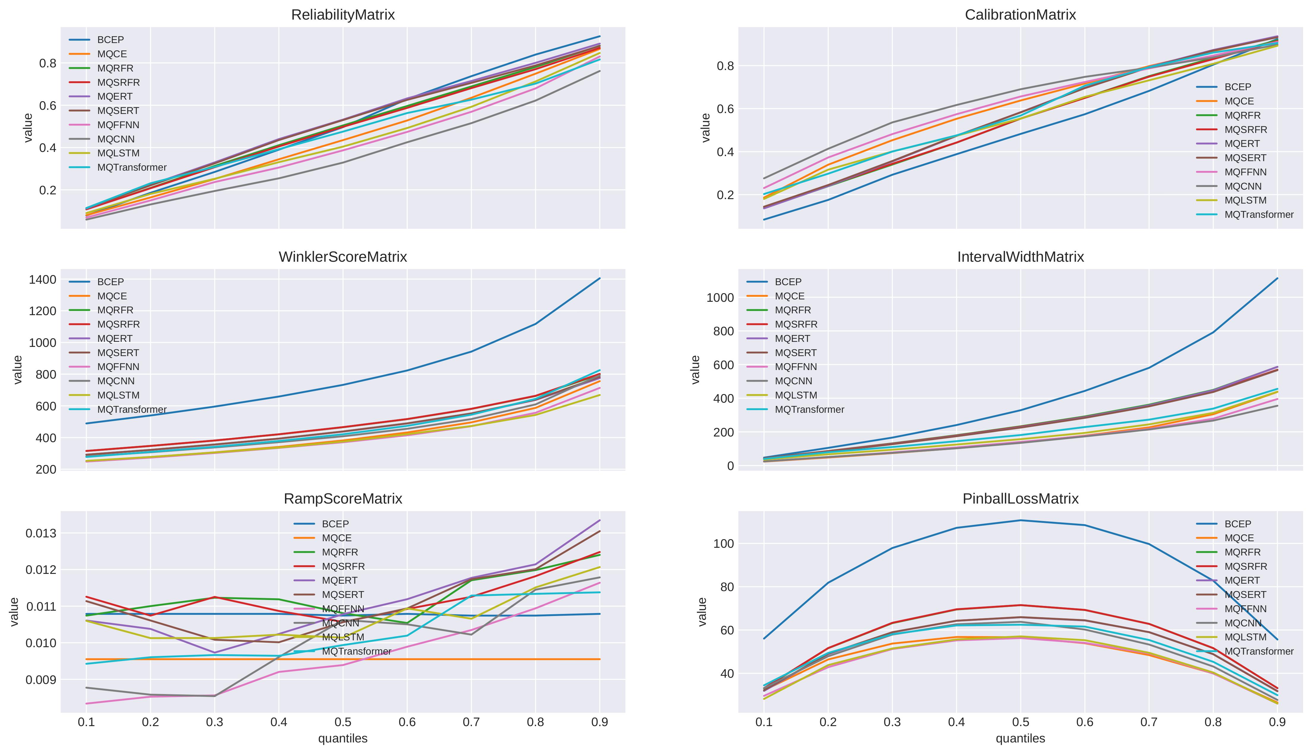
Based on different quantiles, we can give evaluation metrics in matrix form and visualize them to intuitively compare different forecasting methods. The following are relevant visualization examples.